erplots draws exposure-response plots from any model that
implements the [er_model_interface]. This article uses logistic
regression models fitted with erglm, but the plotting code itself has no
knowledge of glm().
Fit the model first
Unlike a plotting function that fits a model behind the scenes, erplots expects you to fit the model yourself and pass it in explicitly:
mod <- erglm_model(ae1 ~ aucss, erglm_data, family = binomial())Defining plots
Basic usage
erglm_data |>
  er_plot(exposure = aucss, response = ae1) |>
  er_plot_show_model(mod) |>
  er_plot_show_quantiles() |>
  plot()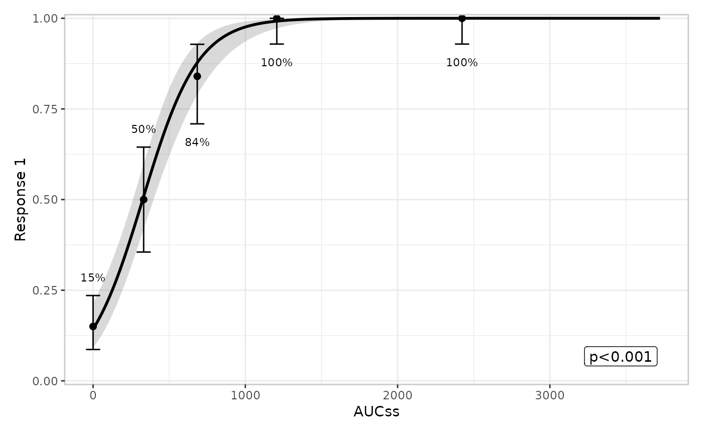
Adding extra components
erglm_data |>
  er_plot(exposure = aucss, response = ae1) |>
  er_plot_show_model(mod) |>
  er_plot_show_quantiles() |>
  er_plot_show_datastrip() |>
  er_plot_show_groups(group_by = aucss) |>
  plot()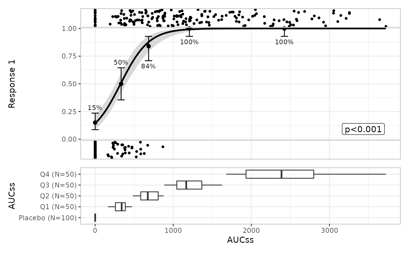
Stratification
Stratification adds colour across all components. This requires a model that includes the stratification variable as a term:
mod_strat <- erglm_model(ae1 ~ aucss + sex, erglm_data, family = binomial())

erglm_data |>
  er_plot(
    exposure = aucss,
    response = ae1,
    stratify_by = sex
  ) |>
  er_plot_show_model(mod_strat) |>
  er_plot_show_quantiles() |>
  er_plot_show_datastrip() |>
  plot()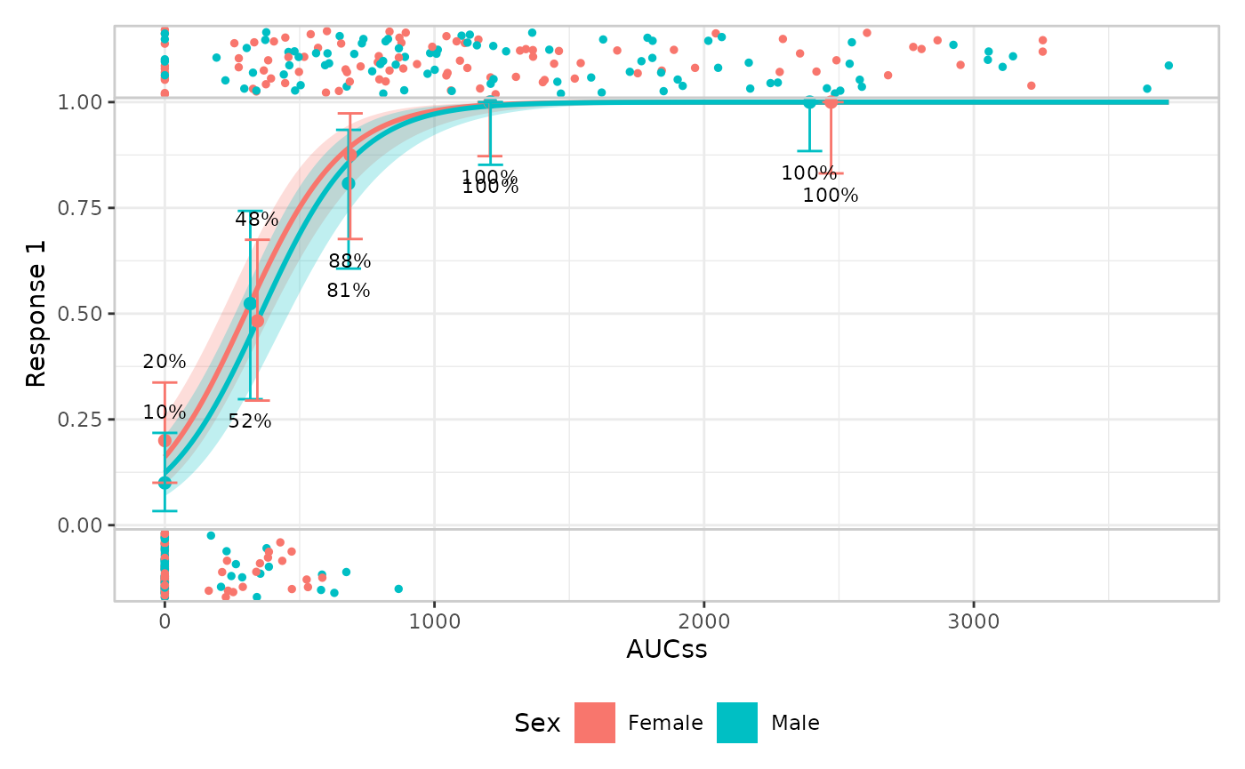
You can suppress stratification for specific components
erglm_data |>
  er_plot(
    exposure = aucss,
    response = ae1,
    stratify_by = sex
  ) |>
  # keep_strata = FALSE needs a model that doesn't include the
  # stratification variable, so we pass the un-stratified `mod` here
  er_plot_show_model(mod, keep_strata = FALSE) |>
  er_plot_show_quantiles() |>
  er_plot_show_datastrip() |>
  plot()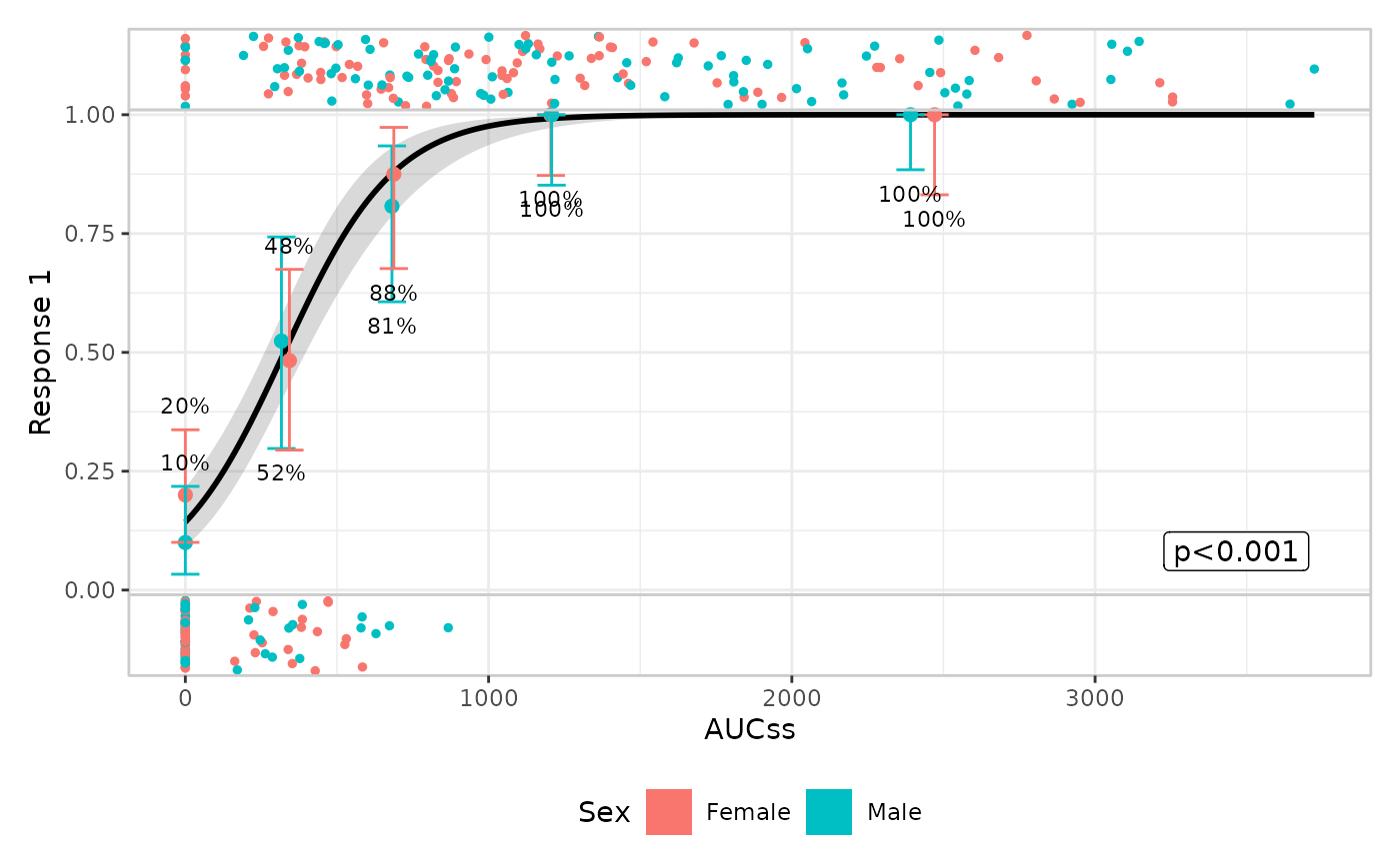
Model component
Default is style = "ribbonline" but you can also draw
spaghetti plots to represent parameter uncertainty. Spaghetti plots
require the model to implement er_simulate() (erglm’s
models do); models that only implement er_predict() fall
back to "ribbonline" with a message.
erglm_data |>
  er_plot(aucss, ae1) |>
  er_plot_show_model(mod, style = "spaghetti") |>
  er_plot_show_quantiles() |>
  plot()
#> Using seed = 4371
#> Warning in ggplot2::geom_path(data = sim, mapping = ggplot2::aes(x =
#> .data[[exposure$name]], : Ignoring unknown parameters: `fill`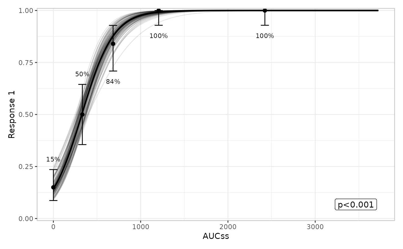
Quantile component
You can modify the number of bins:
erglm_data |>
  er_plot(aucss, ae1) |>
  er_plot_show_model(mod) |>
  er_plot_show_quantiles(bins = 6) |>
  plot()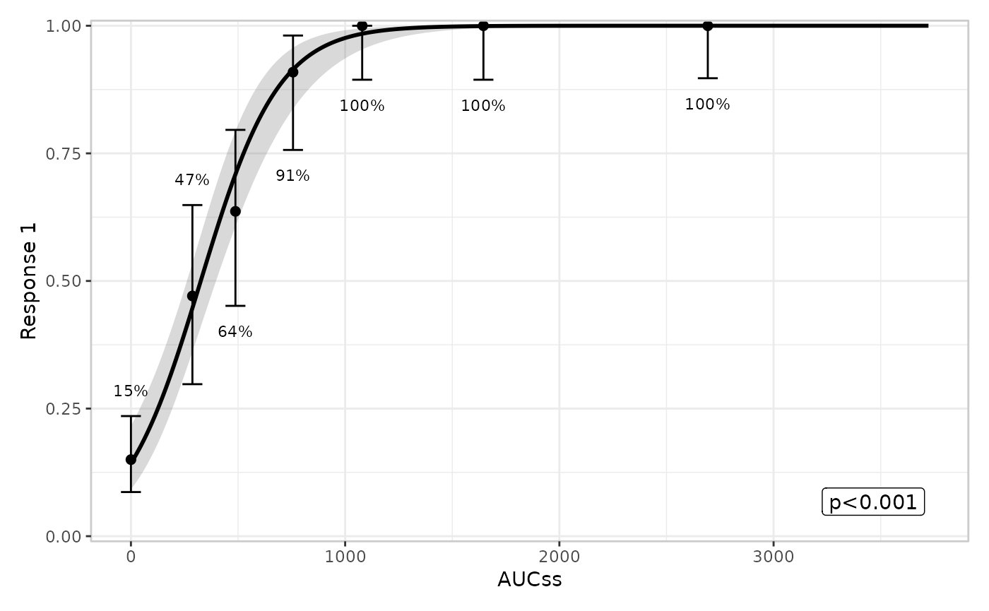
You can also modify the confidence level for the Clopper-Pearson interval (this empirical-summary layer currently assumes a binary response):
erglm_data |>
  er_plot(aucss, ae1) |>
  er_plot_show_model(mod) |>
  er_plot_show_quantiles(bins = 6, conf_level = .8) |>
  plot()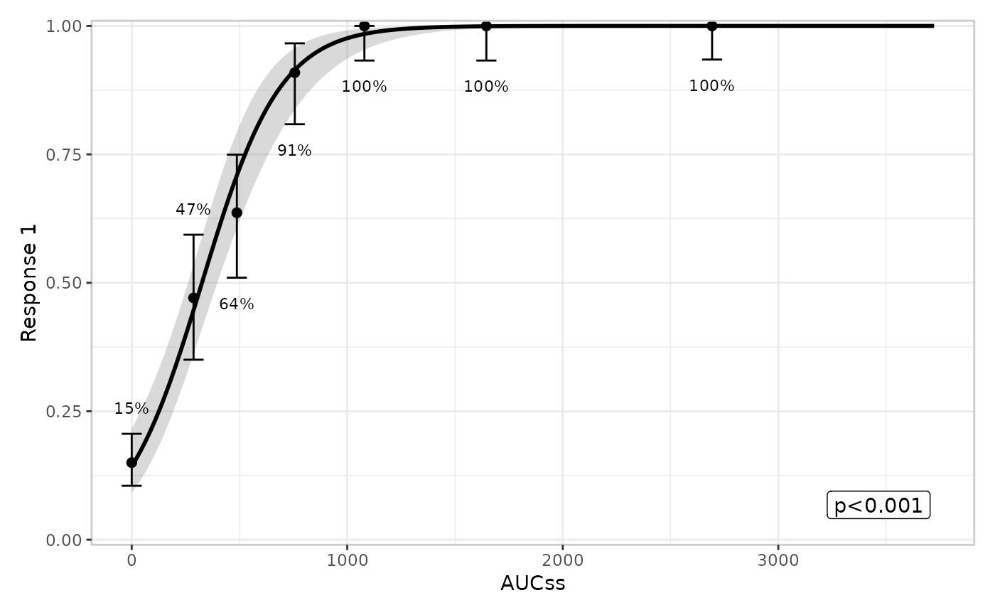
Group component
Multiple grouping variables are allowed:
erglm_data |>
  er_plot(aucss, ae1) |>
  er_plot_show_model(mod) |>
  er_plot_show_quantiles() |>
  er_plot_show_groups(group_by = c(aucss, sex)) |>
  plot()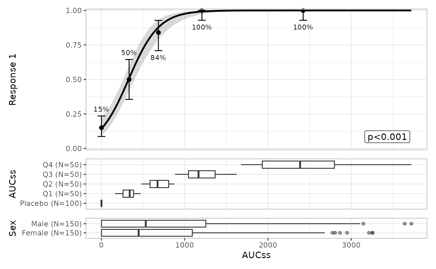
Stratification propagates to the group component:
erglm_data |>
  er_plot(aucss, ae1, stratify_by = sex) |>
  er_plot_show_model(mod_strat) |>
  er_plot_show_quantiles() |>
  er_plot_show_groups(group_by = aucss) |>
  plot()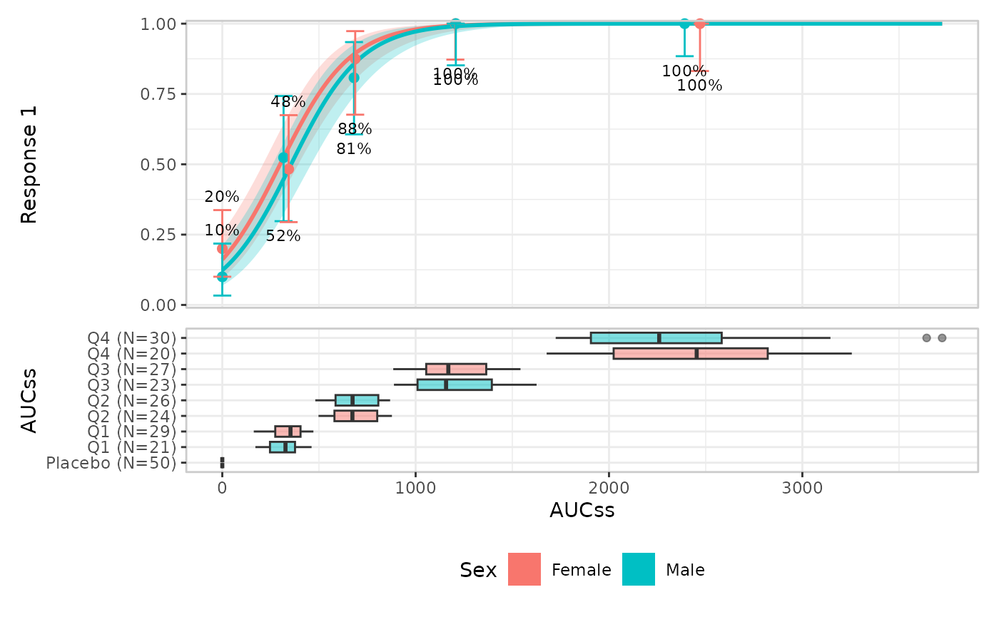
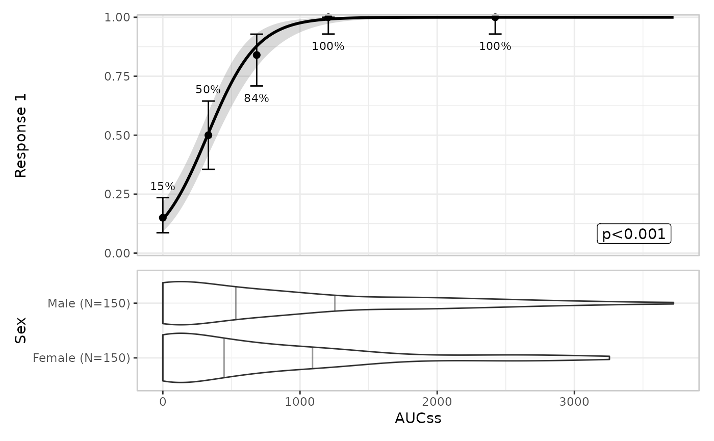
The default is style = "boxplot" but you can also use
violin plots:
erglm_data |>
  er_plot(aucss, ae1) |>
  er_plot_show_model(mod) |>
  er_plot_show_quantiles() |>
  er_plot_show_groups(group_by = sex, style = "violin") |>
  plot()