The exposure-response plotting mini-language

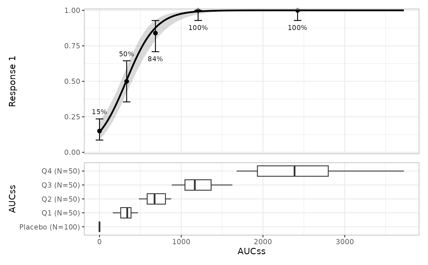
Create an er_plot specification for exposure-response visualization. Build the plot by adding layers (model, summary, quantiles, data, groups) and render with plot()/print() or er_plot_build().

Usage

er_plot(data, exposure, response, stratify_by = NULL, response_type = "auto")

Arguments

data

Data frame or tibble containing the observed data.

exposure

Exposure variable (one variable, unquoted).

response

Response variable (one variable, unquoted).

stratify_by

Stratification variable used for colour and fill (one variable, unquoted).

response_type

One of "auto", "binary", "continuous", or "count".

Value

An (empty) plot object of class er_plot.

Details

Layers are either singleton or additive: model, summary, quantile, and data layers are singleton (a second call replaces the previous); groups are additive (each call adds a panel).

stratify_by declares a discrete variable used for colour/fill across layers; each layer's keep_strata controls whether it uses stratification. Rows with NA in the stratification variable are kept as their own level.

response_type governs response-scale defaults and which interval method the quantile and VPC layers use; see response_type below and er_plot_add_quantiles() for details.

See also

er_plot_add_model(), er_plot_add_summary(), er_plot_add_quantiles(), er_plot_add_data(), er_plot_add_groups(), er_plot_build(), er_plot_theme(), er_model_interface

Examples

if (requireNamespace("erglm", quietly = TRUE)) {
library(erglm)
mod <- erglm_model(ae1 ~ aucss, erglm_data, family = binomial())

erglm_data |>
  er_plot(aucss, ae1) |>
  er_plot_add_model(mod) |>
  er_plot_add_quantiles() |>
  er_plot_add_groups(aucss) |>
  plot()
}