The built plot object (internal structure)

This article documents an implementation detail, not a public interface. Everything described below – the shape of object$plot, object$layer, and object$output, the names used internally, and the internal .polish_*()/.build_*() helpers – is unexported, undocumented in ?er_plot, and not covered by erplots’ usual conventions. It can, and likely will, change in a future release without notice or a deprecation period. Nothing in this article should be relied on in package code, and any script that depends on it should be treated as tied to the erplots version it was written against.

The preferred way to change how a plot looks is a custom style function (see Extending erplots). Read this article only if you’ve hit a case that mechanism genuinely can’t reach – e.g. a one-off tweak to a specific panel’s theme, or a fix you need right now and don’t want to write and register a whole custom builder for – and you’re willing to reach into the object and patch it by hand.

library(erplots)
library(erglm)

mod <- erglm_model(ae1 ~ aucss, erglm_data, family = binomial())

p <- erglm_data |>
  er_plot(aucss, ae1) |>
  er_plot_add_model(mod) |>
  er_plot_add_quantiles() |>
  er_plot_add_data(style = er_style_data_boxjitter)

Two stages: object$plot, then object$output

Calling plot() (or print()) on an er_plot object calls er_plot_build() first. er_plot_build() does its work in two stages, and both intermediate results are kept on the returned object rather than discarded:

built <- er_plot_build(p)
names(built)
#> [1] "data"     "exposure" "response" "strata"   "layer"    "plot"     "theme"   
#> [8] "output"

Stage one builds one ordinary ggplot2 object per layer family, stored under built$plot. Stage two (“polishing”: margins, axis/legend labels, discrete colour scales, panel arrangement, legend deduplication, and the plot-level theme) turns those separate ggplot2 objects into a single patchwork object, stored under built$output. plot.er_plot() itself is little more than

plot.er_plot <- function(x, y = NULL, ...) {
  object <- er_plot_build(x)
  plot(object$output)
}

so built$output is exactly what you see rendered.

object$plot: one ggplot2 object per layer family

built$plot is a plain list with up to three slots – base, data, group – each either NULL or containing real ggplot2 object(s):

names(built$plot)
#> [1] "base"  "data"  "group"
class(built$plot$base)
#> [1] "ggplot2::ggplot" "ggplot"          "ggplot2::gg"     "S7_object"      
#> [5] "gg"

• base is a single ggplot2 object. It carries the model curve/ribbon, the quantile summary geoms, and the summary annotation – whichever of those layers are present – and only exists at all if at least one of them is (or if the plot has no layers whatsoever, in which case it’s an empty axes-only canvas). An "overlay"-layout data builder (the default, er_style_data_overlay()) also draws directly onto base, rather than into its own panel – so a plot built with the default data style has a NULL built$plot$data even though it clearly has a data layer:

  p_overlay <- erglm_data |> er_plot(aucss, ae1) |> er_plot_add_data()
  built_overlay <- er_plot_build(p_overlay)
  names(built_overlay$plot)
  #> [1] "base"  "data"  "group"
  is.null(built_overlay$plot$data)
  #> [1] TRUE

• data is a named list of ggplot2 objects – never a single bare object, even when there’s only one panel – used only by a "panel"-layout data builder (e.g. er_style_data_boxjitter(), used in p above). The names are meaningful and depend on response type and stratification: "upper"/"lower" for the binary responder/non-responder split, "data" for a single unstratified continuous/count panel, or one name per stratum level when stratified and faceted.

  names(built$plot$data)
  #> [1] "upper" "lower"

• group is a named list of ggplot2 objects, one per grouping variable added via er_plot_add_groups(), keyed by variable name. NULL if no group layer was added.

object$output: the final patchwork object

class(built$output)
#> [1] "patchwork"       "ggplot2::ggplot" "ggplot"          "ggplot2::gg"    
#> [5] "S7_object"       "gg"

built$output is what patchwork::wrap_plots() produces from the individual panels in built$plot (stacked vertically via ncol = 1, sized by er_plot_theme()’s height_* arguments, with guides = "collect" and axes = "collect" to merge legends and align axes across panels), plus patchwork::plot_annotation() for the plot-level title/subtitle/caption.

A patchwork object behaves like an ordinary list of its constituent plots for indexing purposes, which is the most direct route to a hand patch: pull out the panel you want, modify it like any ggplot2 object, and put it back.

length(built$output)
#> [1] 3
built$output[[1]] <- built$output[[1]] + ggplot2::labs(title = "Responders")
built$output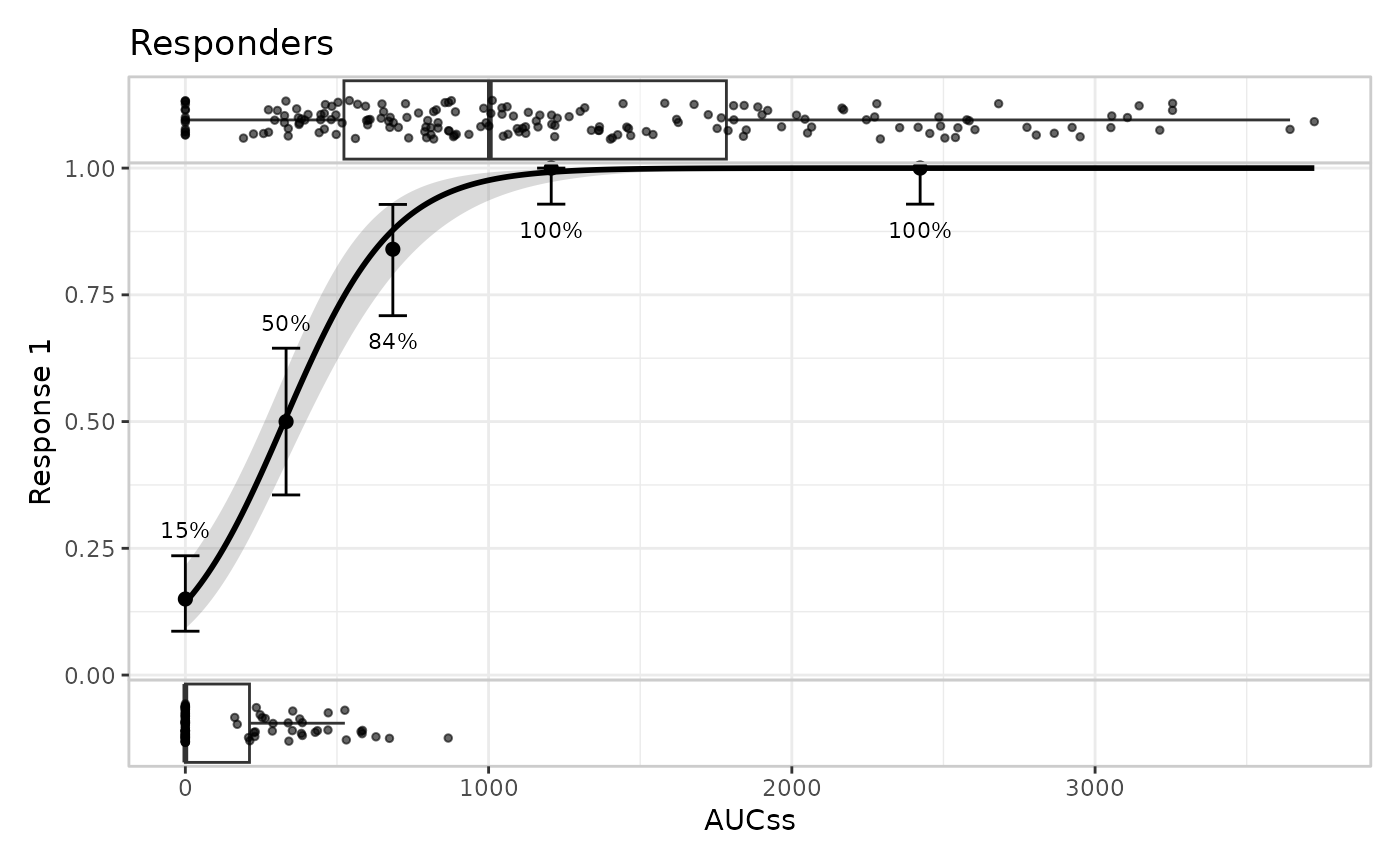

This is usually less error-prone than editing built$plot and re-running the polishing steps yourself, since it works entirely with ordinary, already-composed ggplot2 objects and doesn’t need to know about the internal .polish_*() helpers at all. Its limitation is exactly that it operates after polishing – e.g. adding a new discrete colour mapping this way won’t get the cross-panel legend deduplication that er_plot_theme(color_discrete = ...) gets, because that logic already ran.

Summary

Object	Type	Contains
built$plot$base	single ggplot object, or NULL	model/summary/quantile geoms, and an "overlay"-layout data builder’s points
built$plot$data	named list, or NULL	one panel per "panel"-layout data builder’s output
built$plot$group	named list, or NULL	one panel per er_plot_add_groups() variable
built$output	single patchwork object	all of the above, stacked, themed, and annotated

Treat all of this as a snapshot of the current implementation, not a contract – see the warning at the top of this article.