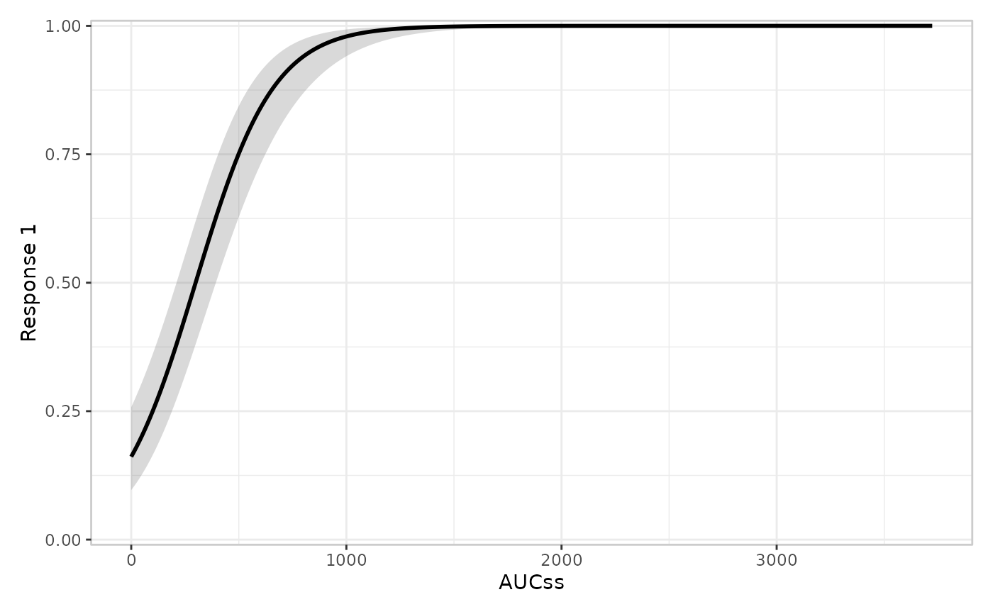
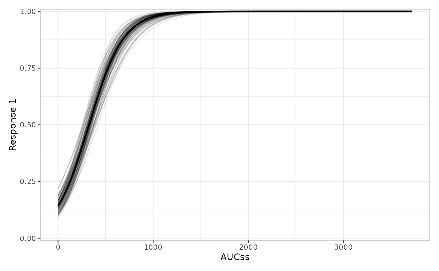
Add a fitted-model curve/ribbon layer

Adds the model layer: a fitted exposure-response curve with an uncertainty ribbon, or possibly a spaghetti plot of simulated draws.

Usage

er_plot_add_model(
  object,
  model,
  style = NULL,
  keep_strata = NULL,
  conf_level = 0.95,
  predict_args = list(),
  ...
)

Arguments

object: Partially constructed plot (has S3 class er_plot).
model: A fitted exposure-response model. Must implement er_predict().
style: Style used to draw the model curve/ribbon layer. Can either be a string corresponding to one of the registered style labels (e.g., "ribbonline", the default), or a builder function used to compute the relevant plot object (see "Styles" below).
keep_strata: Logical; whether this layer should use stratification. Defaults to TRUE when a stratification variable has been specified, and FALSE otherwise.
conf_level: Confidence level for the prediction ribbon. Defaults to 0.95.
predict_args: A named list of additional arguments forwarded to er_predict() when generating model-based predictions.
...: Additional named arguments forwarded to the style builder function when the plot is built.

Value

The input object, with the model layer added.

Details

This layer uses er_predict() to compute model predictions on the response scale. model may reference covariates beyond the exposure and strata variables. erplots fills any additional covariates from the plot data with a reference value (first factor level or numeric mean) when building the prediction grid. erplots does not check that model was fit on the same exposure/response as the plot; the caller must ensure compatibility.

Styles

The following pre-defined styles are available for this layer. Please see the documentation for the corresponding builder function to see what customisation options are available:

Label	Builder	Description
`"ribbonline"`	`er_style_model_ribbonline()`	Fitted curve with an uncertainty ribbon (the default).
`"line"`	`er_style_model_line()`	Fitted curve only, no ribbon.
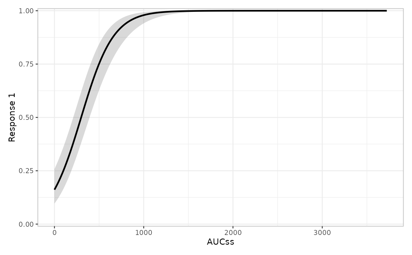
`"spaghetti"`	`er_style_model_spaghetti()`	Fitted curve plus a spaghetti plot of simulated draws, for models implementing `er_simulate()`.

See er_style() for details on how style builder functions are defined for the exposure-response mini-grammar, should a custom style be required.

Examples

if (requireNamespace("erglm", quietly = TRUE)) {
library(erglm)
mod <- erglm_model(ae1 ~ aucss, erglm_data, family = binomial())
erglm_data |>
  er_plot(aucss, ae1) |>
  er_plot_add_model(mod) |>
  plot()

# a spaghetti plot instead of the default ribbon
erglm_data |>
  er_plot(aucss, ae1) |>
  er_plot_add_model(mod, style = er_style_model_spaghetti) |>
  plot()

# the same spaghetti plot, selected by its registered label instead
# (see `?er_style_labels`)
erglm_data |>
  er_plot(aucss, ae1) |>
  er_plot_add_model(mod, style = "spaghetti") |>
  plot()

# plug in a fully custom model-curve builder
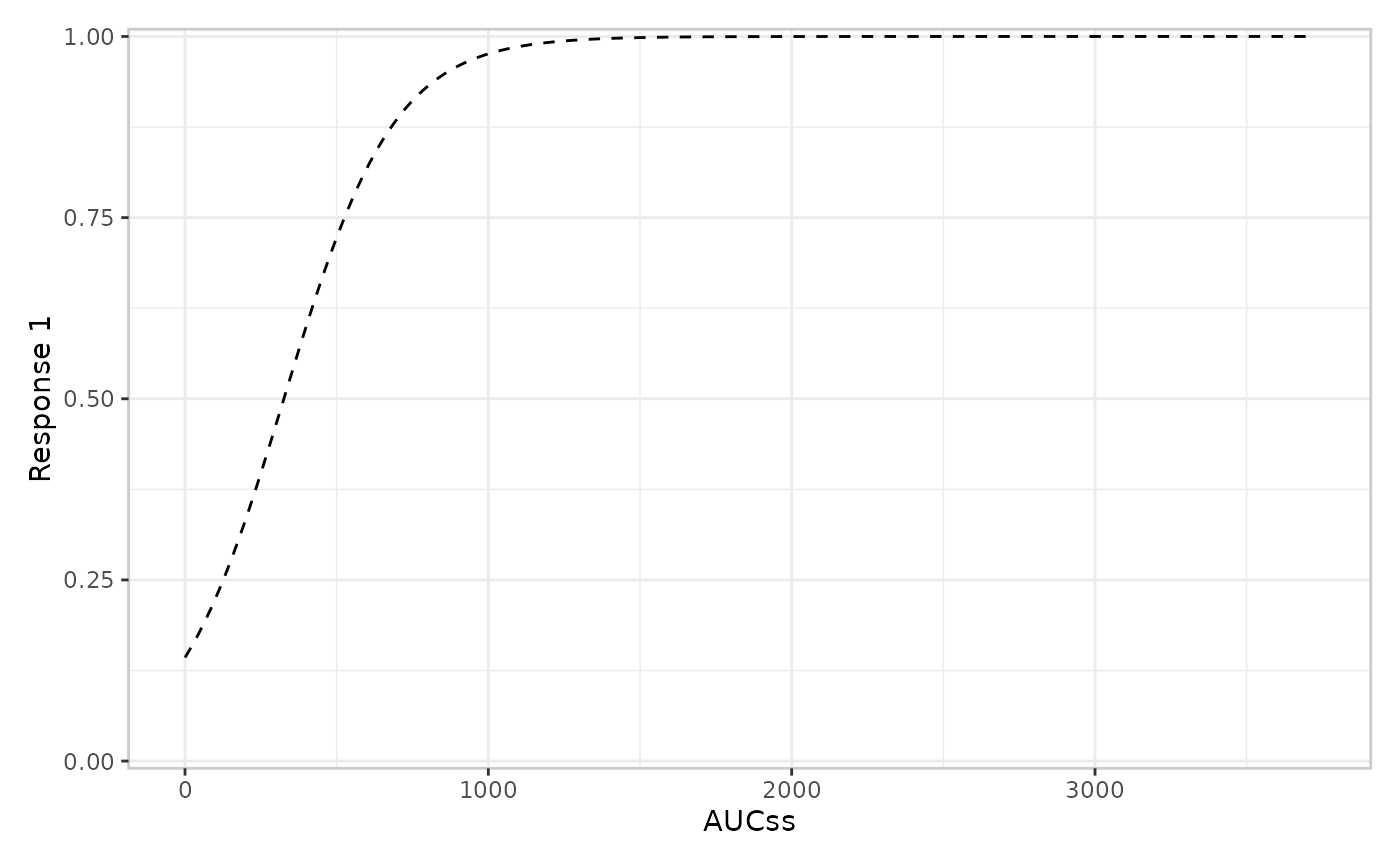
build_model_dashed <- function(data, config, stratify, exposure, response, strata, theme, ...) {
  ggplot2::geom_line(
    data = config$predictions,
    mapping = ggplot2::aes(x = .data[[exposure$name]], y = fit_resp),
    linetype = "dashed"
  )
}
erglm_data |>
  er_plot(aucss, ae1) |>
  er_plot_add_model(mod, style = build_model_dashed) |>
  plot()

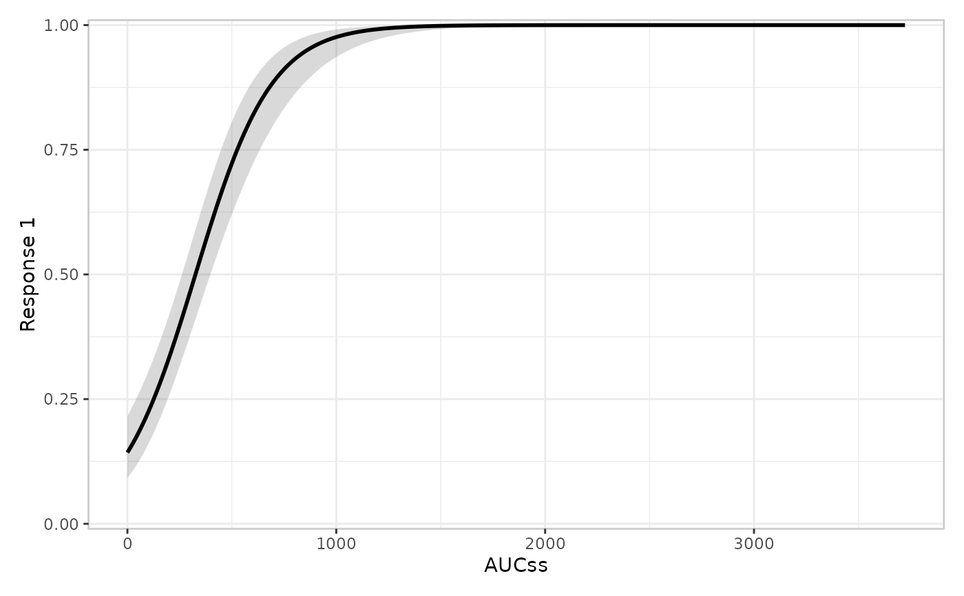
# a model with a covariate beyond the exposure variable still works even when
# this layer isn't stratifying by it: `sex` is set to a reference value
# when building the prediction grid, which may not be what the user wants
mod_sex <- erglm_model(ae1 ~ aucss + sex, erglm_data, family = binomial())
erglm_data |>
  er_plot(aucss, ae1) |>
  er_plot_add_model(mod_sex) |>
  plot()
}

#> Using seed = 3953. Pass `seed = 3953` to reproduce this result.

#> Using seed = 8038. Pass `seed = 8038` to reproduce this result.