Plotting continuous responses

The erplots package supplies a mini-language for generating exposure-response plots commonly used in pharmacometric analyses. It is designed to be model agnostic, in the sense that it will work for any modelling tool that implements a few key interface functions (see Implementing the model interface). It can support binary response data, continuous response data, and count response data. This article focuses on continuous data, using a linear regression model fitted using the erglm package. It covers the substantive aspects of plot construction, not the superficial features like labels, palettes, and visual theme. Those are covered by the theming erplots article, which applies unchanged regardless of response type.

library(erplots)
library(erglm)

Fit the model first

mod_gaussian <- erglm_model(biomarker_change ~ aucss, erglm_data, family = gaussian())

er_plot() auto-detects whether a response is binary (logical, or values entirely in {0, 1}) or continuous, and you can override the detection with response_type. biomarker_change auto-detects as "continuous".

Defining plots

erglm_data |> 
  er_plot(aucss, biomarker_change) |> 
  er_plot_add_model(mod_gaussian) |> 
  er_plot_add_quantiles() |> 
  plot()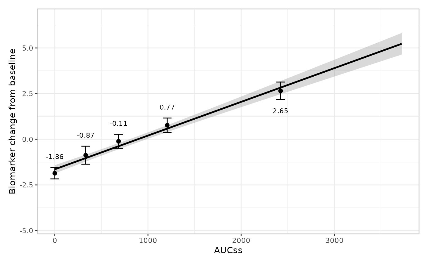

Stratification

Stratification adds colour across all layers, and requires a model that includes the stratification variable as a term. See the binary responses article for a fuller worked example, including how to suppress stratification for specific layers with keep_strata = FALSE.

mod_gaussian_sex <- erglm_model(
  biomarker_change ~ aucss + sex, erglm_data, family = gaussian()
)

erglm_data |> 
  er_plot(aucss, biomarker_change, stratify_by = sex) |> 
  er_plot_add_model(mod_gaussian_sex) |> 
  er_plot_add_quantiles() |> 
  er_plot_add_data() |>
  plot()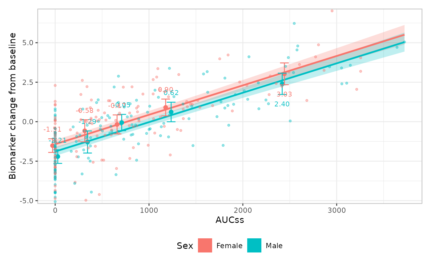

Model layer

The model layer doesn’t look at response_type at all – it only consumes er_predict()/er_simulate() output – so it works exactly the same way as for a binary response. See the binary responses article for er_style_model_spaghetti() and the parameter-uncertainty rationale behind it; the default builder is used here:

erglm_data |> 
  er_plot(aucss, biomarker_change) |> 
  er_plot_add_model(mod_gaussian) |> 
  er_plot_add_quantiles() |> 
  plot()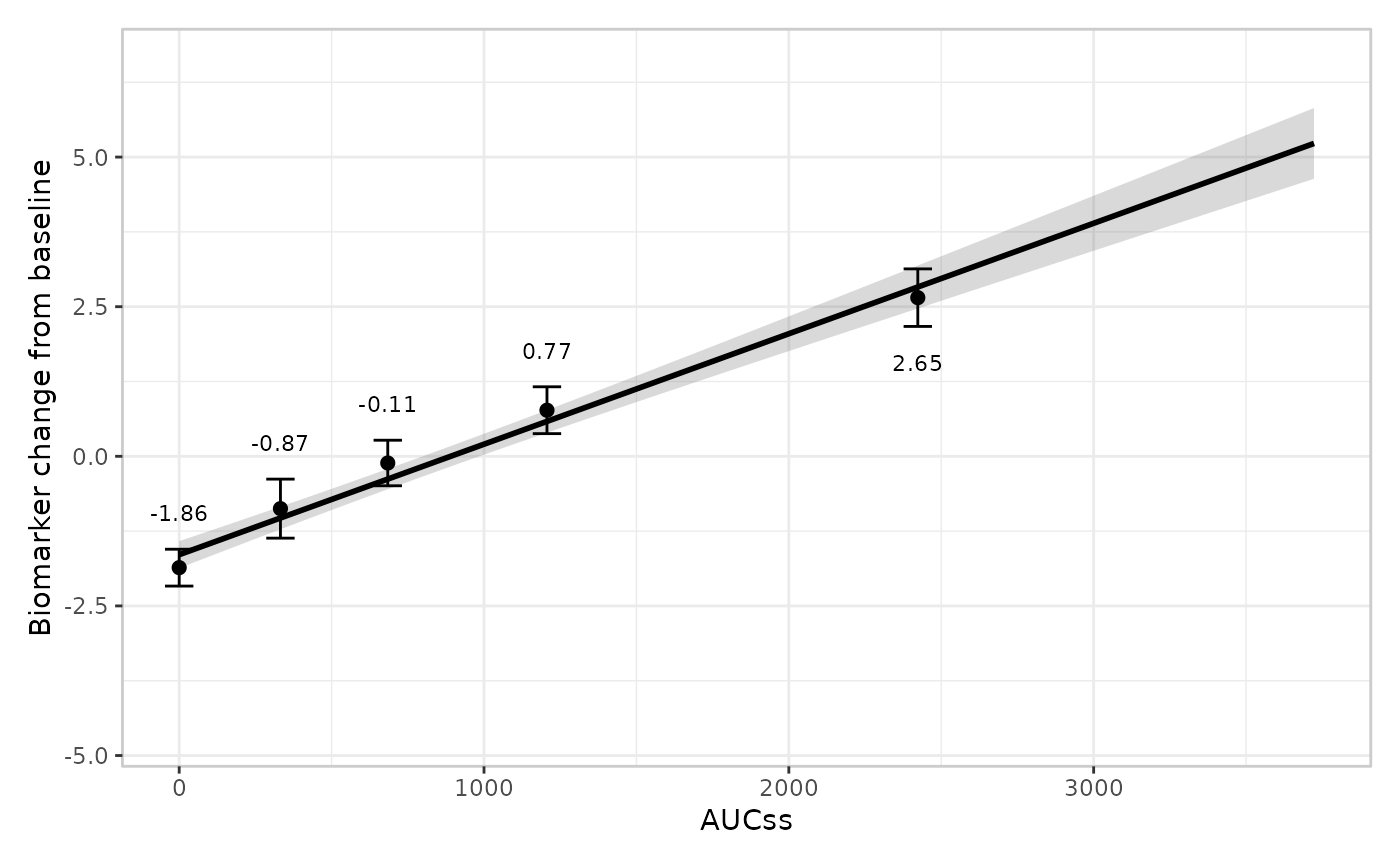

Summary layer

The summary layer doesn’t look at response_type at all either – it only consumes whatever the model’s own er_summary() method returns – so it works exactly the same way as for a binary response. See the binary responses article for er_style_summary_gof() and the full four-builder set; the default builder is used here:

erglm_data |> 
  er_plot(aucss, biomarker_change) |> 
  er_plot_add_model(mod_gaussian) |> 
  er_plot_add_summary(model = mod_gaussian) |> 
  plot()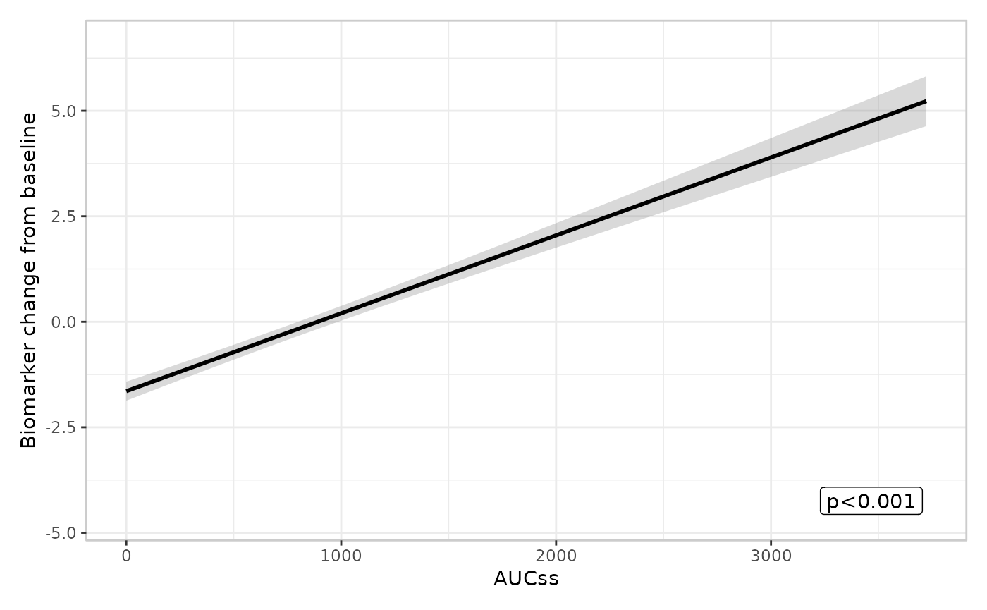

Quantile layer

For a continuous response, each exposure-quantile bin is summarised by its mean with a t-interval, rather than a rate with a Clopper-Pearson interval:

erglm_data |> 
  er_plot(aucss, biomarker_change) |> 
  er_plot_add_model(mod_gaussian) |> 
  er_plot_add_quantiles(bins = 6, conf_level = .8) |> 
  plot()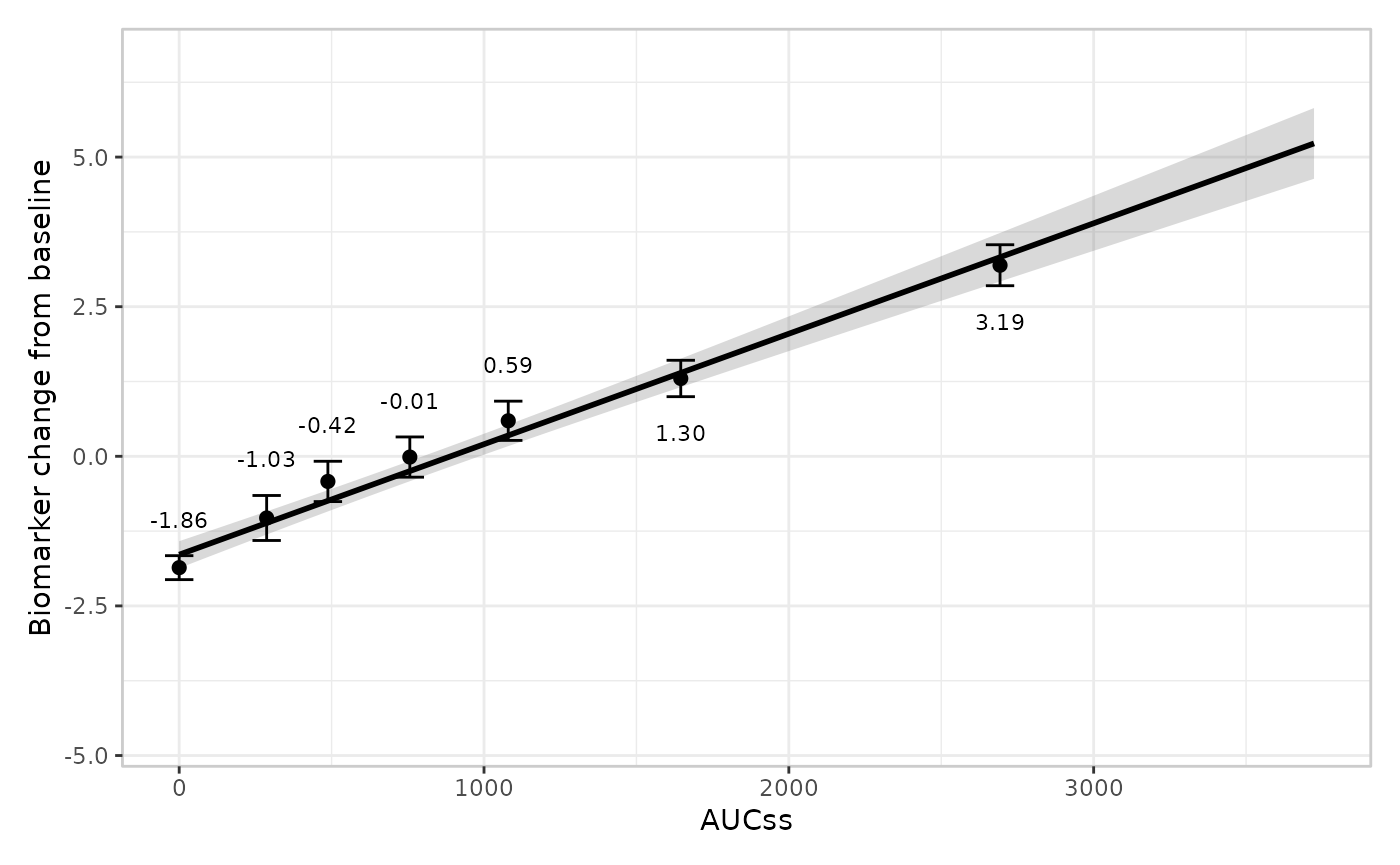

The t-interval is a reasonable default for a genuinely continuous response like this one. See the count responses article for a case – low-count Poisson data – where the t-interval approximation can misbehave (a negative lower bound), and the response_type = "count" declaration that fixes it.

Data layer

er_plot_add_data() adds the raw observations at their true (exposure, response) coordinates via er_style_data_overlay(), the default and only built-in builder for a continuous response – no jitter is needed, since the response isn’t confined to 0/1:

erglm_data |> 
  er_plot(aucss, biomarker_change) |> 
  er_plot_add_model(mod_gaussian) |> 
  er_plot_add_data() |> 
  plot()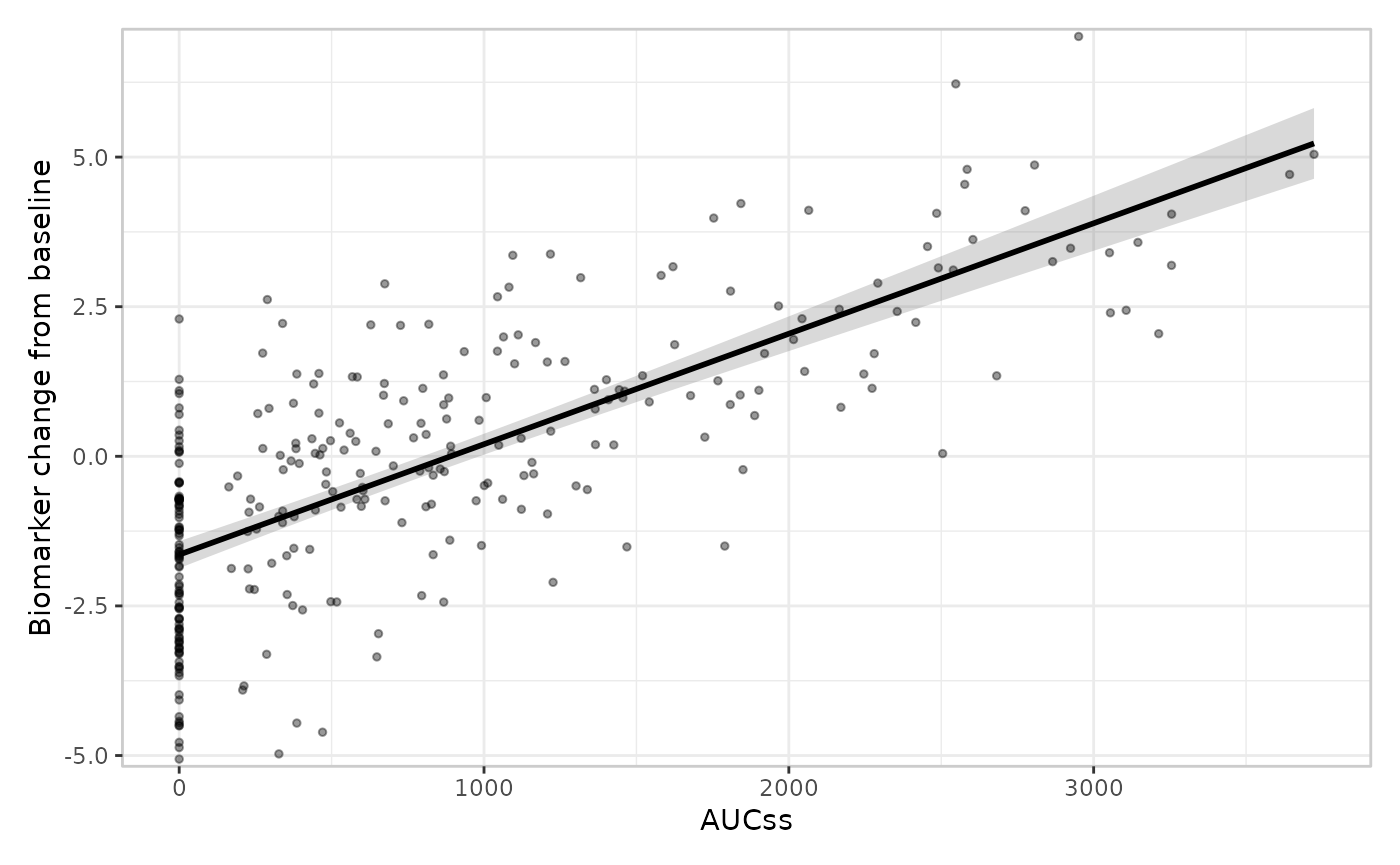

There’s no built-in panel-based alternative for a continuous response – er_style_data_boxjitter() (the panel-based responders/non-responders design covered in the binary responses article) is binary-only. If you need a panel-based builder here (e.g. a single colour-encoded panel), you can write a custom one and tag it with er_style_tag(fn, layout = "panel") – see the Extending erplots article.

Group layer

The group layer doesn’t look at response_type at all – it only consumes the exposure variable – so it works exactly the same way as for a binary response. See the binary responses article for multiple grouping variables and er_style_group_violin(); the default builder and a single grouping variable are shown here:

erglm_data |> 
  er_plot(aucss, biomarker_change) |> 
  er_plot_add_model(mod_gaussian) |> 
  er_plot_add_quantiles() |>
  er_plot_add_groups(group_by = aucss) |> 
  plot()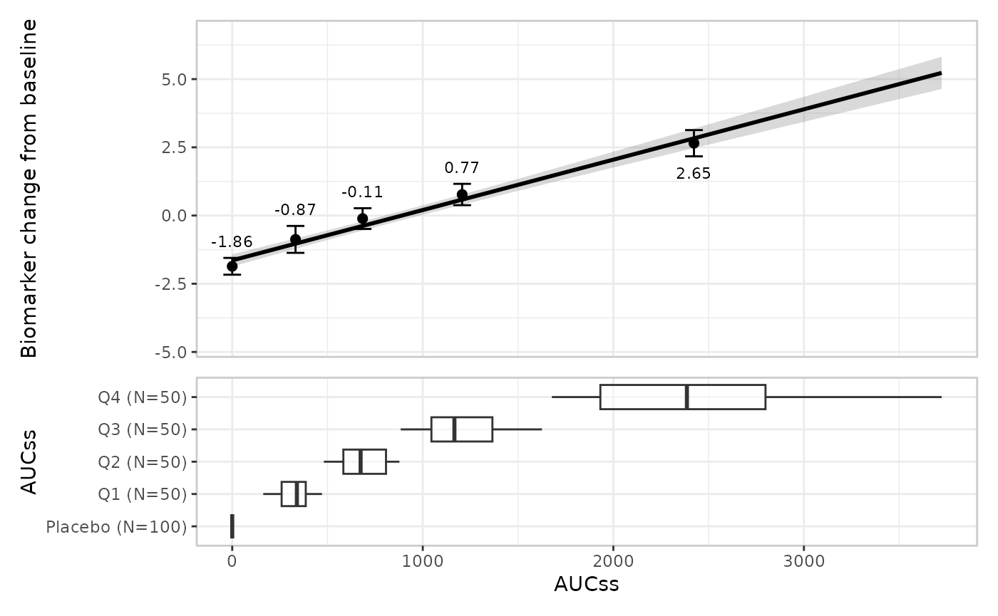

A second model package: emaxnls

Everything above uses erglm’s GLM-based models. To underline that erplots genuinely doesn’t know or care which package fitted the model, here’s the same pipeline driven by an Emax (sigmoidal dose-response) model fitted with emaxnls, which registers its own er_predict()/er_simulate()/er_summary() methods:

library(emaxnls)

mod_emax <- emax_nls(
  structural_model = rsp_1 ~ exp_1,
  covariate_model  = list(E0 ~ 1, Emax ~ 1, logEC50 ~ 1),
  data             = emax_df
)

emax_df |> 
  er_plot(exp_1, rsp_1) |> 
  er_plot_add_model(mod_emax) |> 
  er_plot_add_summary(model = mod_emax, style = er_style_summary_coefficients) |> 
  er_plot_add_quantiles() |> 
  er_plot_add_data() |> 
  plot()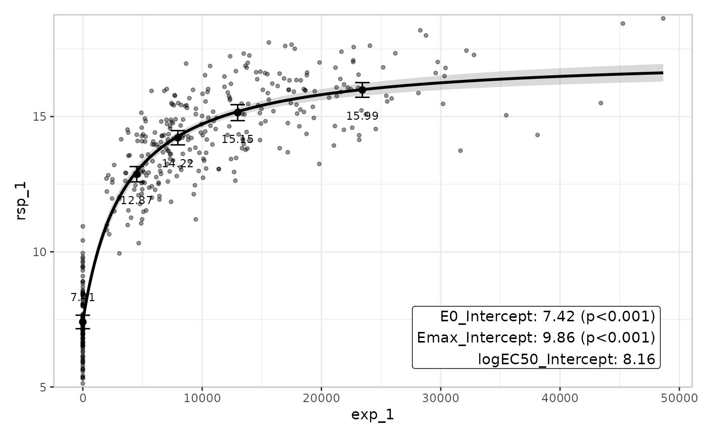

er_style_summary_coefficients() is used here instead of the default er_style_summary_pvalue() because an Emax model has no single privileged coefficient to headline – er_summary.emaxnls() reports p_value = NULL and returns one row per parameter (E0, Emax, logEC50) in coefficients instead.

emaxnls also implements the interface for emax_logistic() models (binary responses). In R’s object-oriented terms, an emaxlogistic object carries class c("emaxlogistic", "emaxnls"), so it automatically reuses the same er_predict()/er_simulate()/er_summary() methods written for a plain emaxnls object (a mechanism called S3 inheritance), rather than emaxnls needing to write a second, separate set of methods. Those shared methods branch internally to keep predictions in [0, 1] and report r_squared = NA (rather than a meaningless value) in er_summary()’s glance whenever they’re handed an emaxlogistic object specifically. None of this detail matters for using emax_logistic() with erplots – fitting one and passing it to er_plot_add_model() just works, the same as any other model. See the binary responses article for that response type in general.