Implementing the model interface

erplots never fits a model. Every plot it draws is built from predictions, simulations, or summary statistics that some other object hands it, via four S3 generics: er_predict(), er_simulate(), er_summary(), and er_predict_survival(). Collectively these are “the model interface”, documented tersely at ?er_model_interface. This article exists because that help topic is a contract, not a tutorial: it tells you what each generic must return, but not what implementing one actually looks like, or why the contract is shaped the way it is. If you maintain a modelling package and want its model objects to work with er_plot_add_model() and friends – or, for a time-to-event model specifically, with er_tte_add_model() – this is the article to read.

You’re assumed to already know your way around S3 dispatch, predict() methods, and the general shape of a modelling package – this article doesn’t re-explain those. What it does explain is the erplots-specific part: which of the four generics to implement, what each one is for, and what erplots does with the result once you’ve implemented it.

library(erplots)
library(erglm)

Why a generic interface at all?

Exposure-response plots need model predictions, but “model predictions” means something different depending on what fit the model: a glm’s predict(type = "response"), an nls object’s own delta-method standard errors, a Bayesian model’s posterior draws. erplots doesn’t want to know about any of that – it wants one stable shape it can build a geom_ribbon() from, regardless of what produced it. er_predict() is that shape. The same reasoning extends to er_simulate() (uncertainty visualisation) and er_summary() (annotation text): each is a narrow, specific question erplots needs answered, phrased so that any model object can answer it by implementing one S3 method.

Only er_predict() is required. er_simulate() and er_summary() are opt-in: their default methods return NULL, which every part of erplots that calls them treats as “not available” rather than an error. A model package can implement just er_predict() and get the model curve/ribbon layer working; adding er_simulate() unlocks spaghetti plots and VPCs; adding er_summary() unlocks p-value/coefficient/goodness-of-fit annotations. None of the three depends on any other being implemented.

er_predict_survival() sits apart from these three: it has nothing to do with er_plot()/er_vpc() at all, and only matters if your model should also plug into er_tte_add_model()’s survival-curve overlay in the separate er_tte() mini-grammar. It has no NULL-returning default either – a model with no survival-curve support should simply not implement it, and er_tte_add_model() errors informatively if it’s called with one anyway.

er_predict(): the one you must write

er_predict(model, newdata, conf_level = 0.95, ...)

Given a fitted model and a newdata data frame of covariate values, return newdata with three columns added: fit_resp (the point prediction, on the response scale), ci_lower, and ci_upper (a conf_level confidence interval around it, also on the response scale). Nothing else is required – no particular column order, no class on the return value, no restriction on what other columns newdata may already have (erplots doesn’t touch them).

Two things are worth calling out explicitly because they’re easy to get wrong:

• The interval is on the response scale, not the link scale. For a binary-response GLM this matters: computing the interval on the linear predictor and then back-transforming with the inverse link gives an asymmetric, properly-bounded-in-[0, 1] interval; computing it directly on the fitted probabilities does not. Get this right at the source, since erplots has no way to tell (or fix) an interval that was computed on the wrong scale.
• newdata is returned, not just used. er_predict()’s contract is “augment and return newdata”, not “return a new three-column data frame”. This matters when newdata carries a stratification column – erplots builds newdata as an exposure grid crossed with every stratum level when the plot is stratified, and expects that column to survive the round trip through er_predict() unchanged.

Arguments beyond model/newdata/conf_level

The fixed signature above covers every model this article’s two toy classes need, but some models need something else entirely – a landmark time for a model that reduces a survival curve to P(event by t*), say, with nowhere else in er_predict(model, newdata, conf_level, ...)’s contract for that value to live. That’s what the trailing ... in the generic’s own signature is for: implement your method as er_predict.your_class(model, newdata, conf_level = 0.95, landmark_time = NULL, ...), and a caller reaches it via er_plot_add_model()’s predict_args argument, kept deliberately separate from that same function’s own ... (which reaches the style builder instead – see Extending erplots):

er_plot_add_model(your_model, predict_args = list(landmark_time = 90))

A worked example

Suppose you’re writing a small modelling package of your own. You fit models with a thin wrapper around stats::glm(), and want those model objects to work with erplots. Tag the class first, so dispatch has something to catch:

fit_toy_model <- function(formula, data, family = gaussian()) {
  fit <- glm(formula, data = data, family = family)
  class(fit) <- c("toy_model", class(fit))
  fit
}

mod <- fit_toy_model(ae1 ~ aucss, erglm_data, family = binomial())
class(mod)
#> [1] "toy_model" "glm"       "lm"

Prepending "toy_model" (rather than replacing the class vector) keeps every existing glm/lm method – predict(), summary(), coef(), vcov() – working via ordinary S3 inheritance; er_predict.toy_model() only needs to add the three columns erplots wants, using stats::predict.glm() to do the actual work:

er_predict.toy_model <- function(model, newdata, conf_level = 0.95, ...) {
  z <- -qnorm((1 - conf_level) / 2)
  link <- predict(model, newdata = newdata, se.fit = TRUE, type = "link")
  linkinv <- family(model)$linkinv

  newdata$fit_resp <- linkinv(link$fit)
  newdata$ci_lower <- linkinv(link$fit - z * link$se.fit)
  newdata$ci_upper <- linkinv(link$fit + z * link$se.fit)
  newdata
}

That’s the whole method. It’s already enough to plug into the mini language:

erglm_data |>
  er_plot(aucss, ae1) |>
  er_plot_add_model(mod) |>
  plot()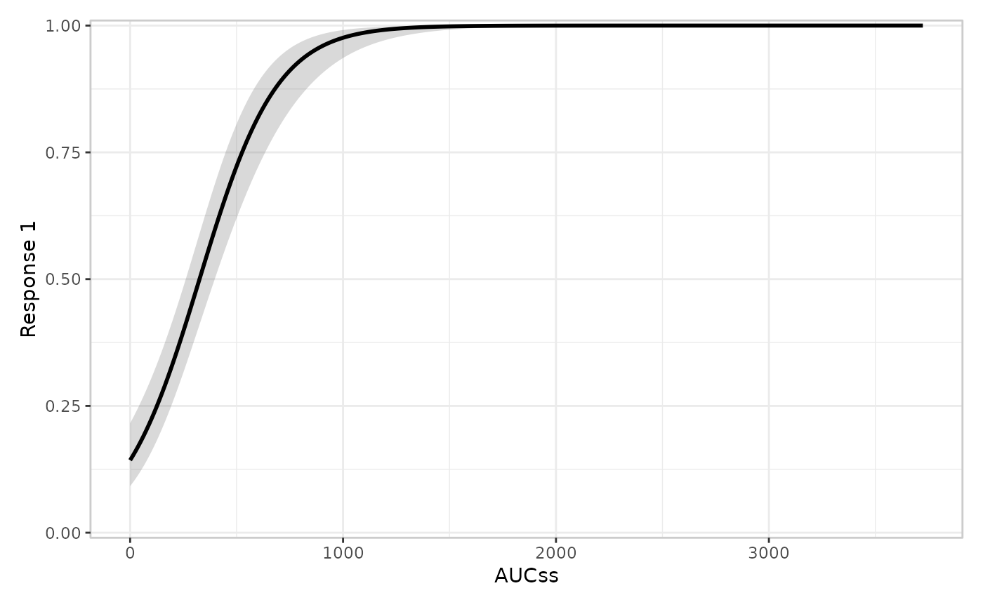

Not every model has a predict() method that computes standard errors for you, though. An nls fit doesn’t – predict.nls() silently ignores se.fit. When there’s no ready-made standard error, the delta method (a numerical gradient of the fitted-value function with respect to the parameters, combined with the parameter covariance matrix) is a general-purpose fallback that works for any differentiable mean function:

emax_fun <- function(par, aucss) {
  par[["e0"]] + par[["emax"]] * aucss / (par[["ec50"]] + aucss)
}

er_predict.toy_emax <- function(model, newdata, conf_level = 0.95, ...) {
  z <- -qnorm((1 - conf_level) / 2)
  par <- coef(model)
  fit <- emax_fun(par, newdata$aucss)

  eps <- 1e-6
  grad <- vapply(names(par), function(nm) {
    par_up <- par; par_up[nm] <- par_up[nm] + eps
    par_dn <- par; par_dn[nm] <- par_dn[nm] - eps
    (emax_fun(par_up, newdata$aucss) - emax_fun(par_dn, newdata$aucss)) / (2 * eps)
  }, FUN.VALUE = numeric(nrow(newdata)))
  se <- sqrt(rowSums((grad %*% vcov(model)) * grad))

  newdata$fit_resp <- fit
  newdata$ci_lower <- fit - z * se
  newdata$ci_upper <- fit + z * se
  newdata
}

emax_mod <- nls(
  biomarker_change ~ e0 + emax * aucss / (ec50 + aucss),
  data = erglm_data,
  start = list(e0 = -2, emax = 5, ec50 = 1000)
)
class(emax_mod) <- c("toy_emax", class(emax_mod))

erglm_data |>
  er_plot(aucss, biomarker_change) |>
  er_plot_add_model(emax_mod) |>
  plot()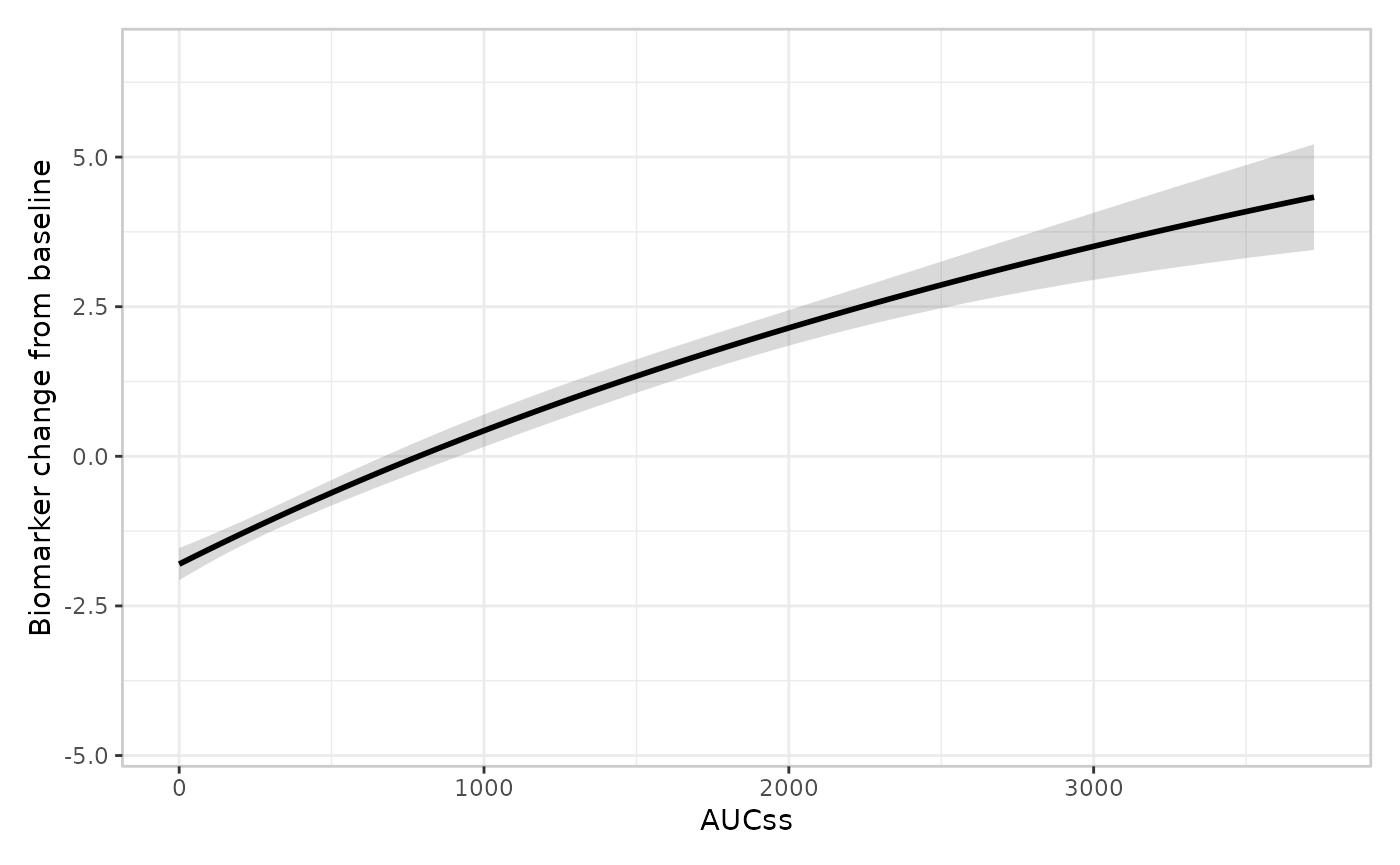

This emax_fun()/finite-difference pairing is deliberately hand-rolled, to keep this article dependency-free; a real implementation would more likely reach for numDeriv::jacobian(), or – if the fitting function already has an analytic gradient available (as nls() itself does, internally) – use that instead of finite differences.

A worked example: an argument beyond the fixed contract

To see predict_args actually reach a method, extend toy_model with a landmark-style transform: a (deliberately simplistic) rescaling of the fitted probability by how far a caller-supplied landmark_time is from a fixed reference. landmark_time has no slot in er_predict()’s fixed model/newdata/conf_level contract, so it can only arrive through ...:

er_predict.toy_landmark <- function(model, newdata, conf_level = 0.95, landmark_time = NULL, ...) {
  if (is.null(landmark_time)) {
    rlang::abort("`er_predict.toy_landmark()` requires `landmark_time`.")
  }
  out <- er_predict.toy_model(model, newdata, conf_level = conf_level)
  scale <- landmark_time / 90
  out$fit_resp <- pmin(out$fit_resp * scale, 1)
  out$ci_lower <- pmin(out$ci_lower * scale, 1)
  out$ci_upper <- pmin(out$ci_upper * scale, 1)
  out
}

landmark_mod <- mod
class(landmark_mod) <- c("toy_landmark", class(landmark_mod))

Omitting landmark_time errors, rather than silently plotting an unscaled curve:

erglm_data |>
  er_plot(aucss, ae1) |>
  er_plot_add_model(landmark_mod) |>
  plot()
#> Error:
#> ! `er_predict.toy_landmark()` requires `landmark_time`.

Supplying it via predict_args reaches the method – and, since landmark_time genuinely changes what’s plotted (a shorter landmark means a lower probability of the event having happened by then), a smaller value visibly flattens the curve:

erglm_data |>
  er_plot(aucss, ae1) |>
  er_plot_add_model(landmark_mod, predict_args = list(landmark_time = 30)) |>
  plot()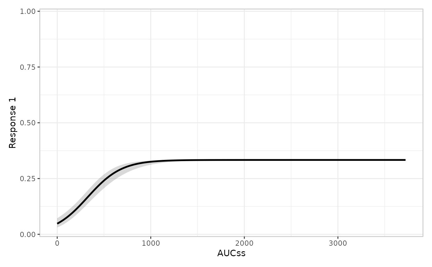

The same predict_args list happily coexists with a style builder that has its own, unrelated extra arguments via ... – the two never collide, because they’re spliced into two different calls (er_predict() and style, respectively):

erglm_data |>
  er_plot(aucss, ae1) |>
  er_plot_add_model(
    landmark_mod,
    style = "spaghetti",
    predict_args = list(landmark_time = 90),
    seed = 8213
  ) |>
  plot()
#> `er_simulate()` is not implemented for objects of class
#> <toy_landmark/toy_model/glm/lm>; falling back to `style =
#> er_style_model_ribbonline`.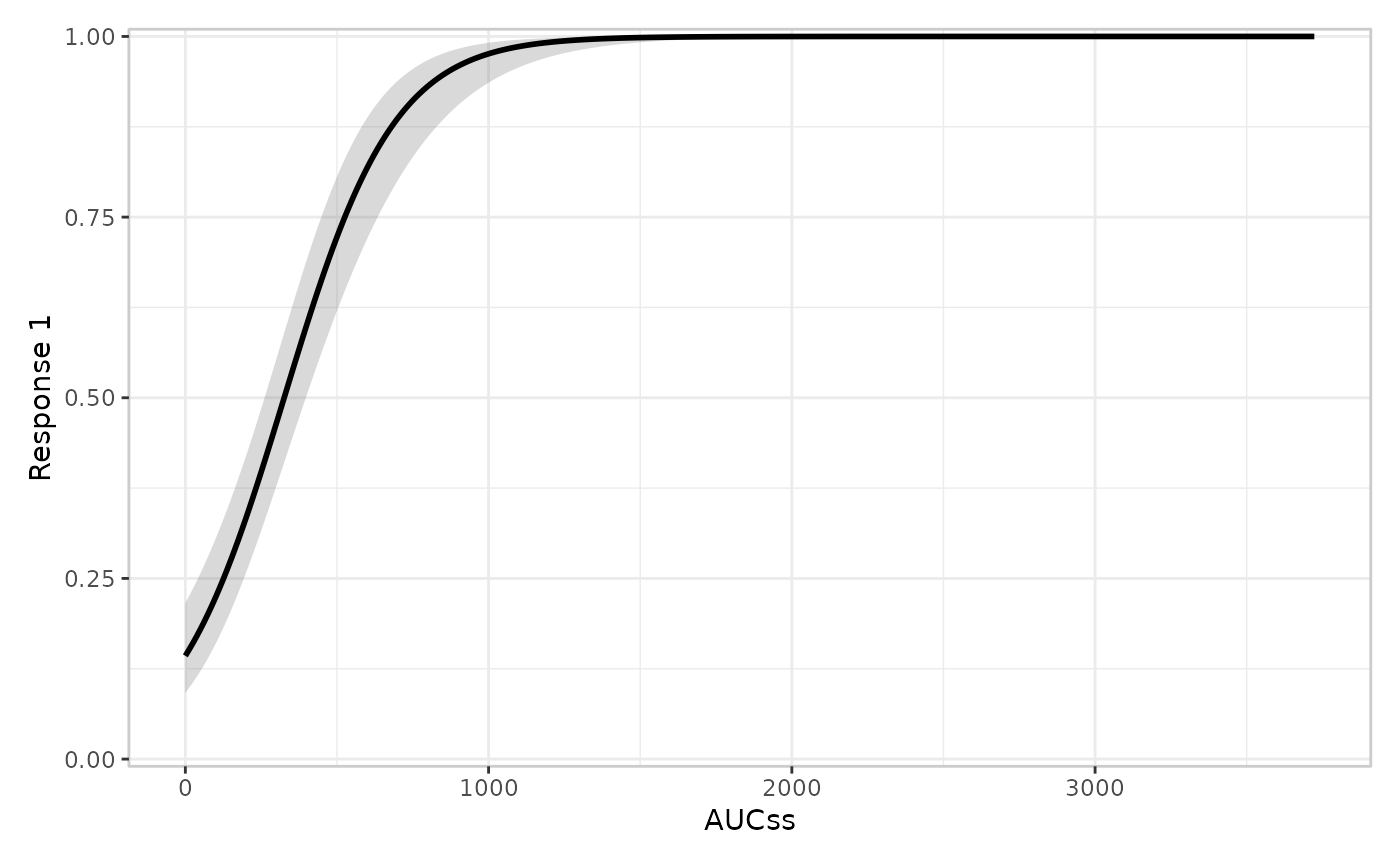

er_plot_add_summary()’s summary_args and er_vpc_add_simulated()’s simulate_args work the same way, for er_summary()/er_simulate() methods that need an argument beyond what’s covered below.

er_simulate(): for spaghetti plots and VPCs

er_simulate(model, newdata, nsim = 100, seed = NULL, ...)

Return a data frame of nsim replicates of newdata, stacked row-wise, with a sim_id column identifying which replicate each row belongs to, and a fit_resp column giving that replicate’s simulated prediction. Don’t implement this generic at all if your model can’t support it – the default method returns NULL, and every caller (er_style_model_spaghetti(), er_vpc_add_simulated()) checks for NULL and treats it as “simulation isn’t available for this model”, not an error.

The one subtlety worth understanding is that fit_resp here means something narrower than it sounds like. It’s a draw from the parameter uncertainty in the model – “if the true parameters were slightly different (as they plausibly could be, given how much data you fit on), where would the mean curve sit?” – not a draw of an actual observation. That’s enough for a spaghetti plot, where every faint line is one plausible mean curve. It is not enough for a visual predictive check, which needs to compare simulated observations (with all their sampling noise) against observed ones – a materially different, noisier quantity. er_simulate()’s contract has an independently optional second column for exactly this, sim_resp: a full response-scale draw that adds observation-level noise on top of the parameter draw (a 0/1 draw for a binary response, an integer draw for a count response, a draw that includes residual variance for a continuous response). A method can return fit_resp alone, or both columns from the same call; there’s no reason to compute sim_resp if you only care about spaghetti plots, but er_vpc_add_simulated(model = ...) will refuse to run (with an informative error, not a silently-too-narrow VPC band) if sim_resp is missing.

A worked example

Continuing the toy_model class from above – drawing parameter vectors from a multivariate normal approximation to the sampling distribution of coef(model) is the standard move for a GLM, and gives you fit_resp for free once you have the draws:

er_simulate.toy_model <- function(model, newdata, nsim = 100, seed = NULL, ...) {
  if (!is.null(seed)) set.seed(seed)

  beta_hat <- coef(model)
  beta_draws <- mvtnorm::rmvnorm(nsim, mean = beta_hat, sigma = vcov(model))
  linkinv <- family(model)$linkinv
  X <- model.matrix(delete.response(terms(model)), data = newdata)

  reps <- vector("list", nsim)
  for (i in seq_len(nsim)) {
    eta <- as.vector(X %*% beta_draws[i, ])
    fit_resp <- linkinv(eta)
    reps[[i]] <- newdata |>
      dplyr::mutate(
        sim_id = i,
        fit_resp = fit_resp,
        # the extra ingredient `sim_resp` needs beyond `fit_resp`:
        # observation-level sampling noise, appropriate to the response
        # type (here, a binary draw at the simulated probability)
        sim_resp = rbinom(length(fit_resp), size = 1, prob = fit_resp)
      )
  }
  dplyr::bind_rows(reps)
}

With this in place, both the spaghetti plot and the VPC work:

erglm_data |>
  er_plot(aucss, ae1) |>
  er_plot_add_model(mod, style = "spaghetti", seed = 8213) |> 
  plot()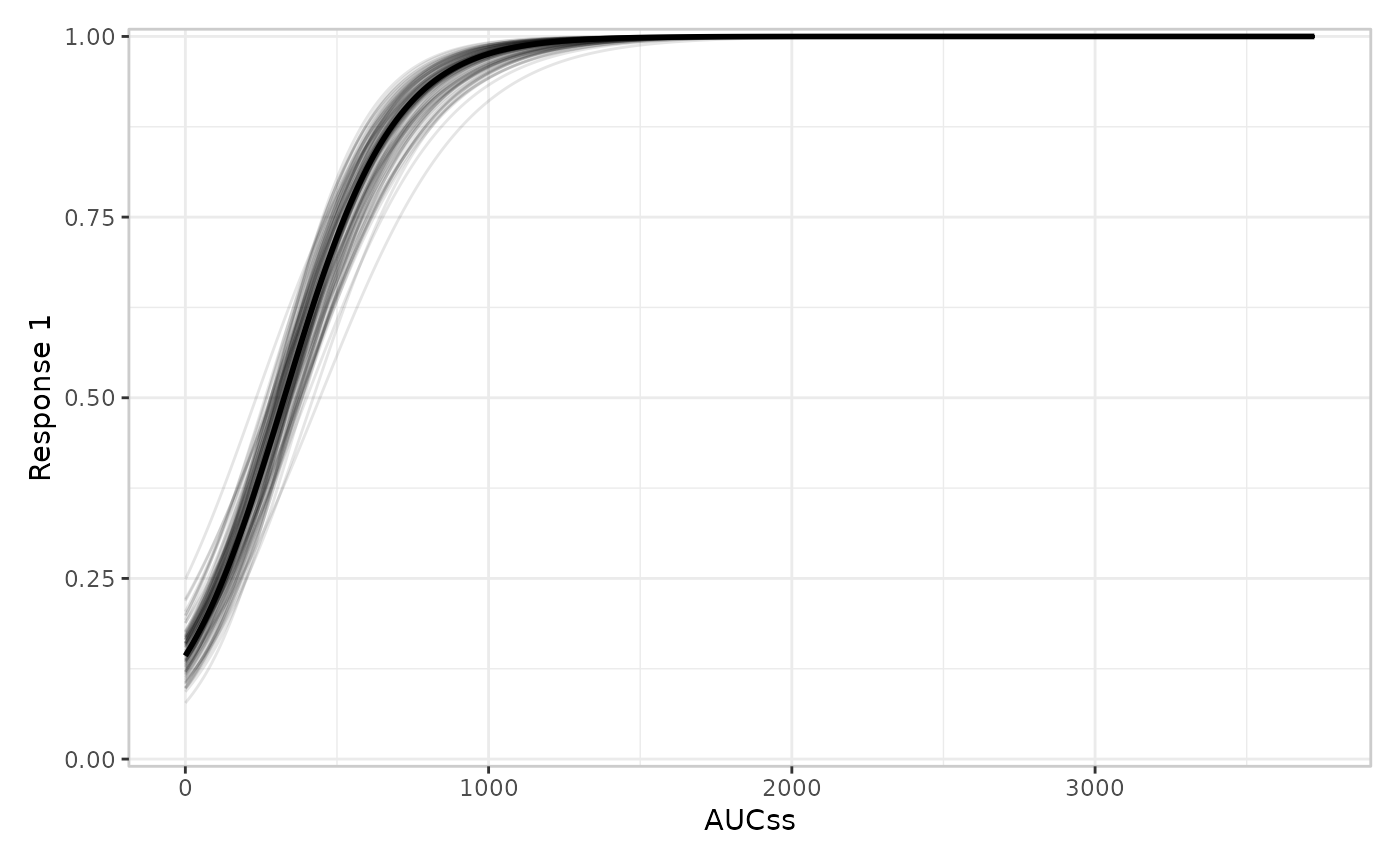

erglm_data |>
  er_vpc(aucss, ae1) |>
  er_vpc_add_observed() |>
  er_vpc_add_simulated(model = mod, nsim = 50, seed = 4471) |>
  plot()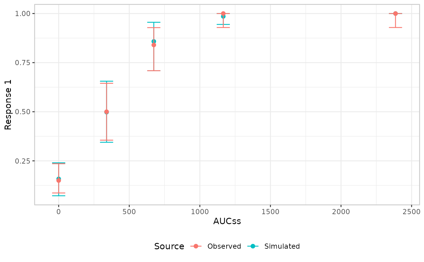

Had er_simulate.toy_model() only ever populated fit_resp, the spaghetti plot above would still work unchanged, but the er_vpc_add_simulated() call would error, naming sim_resp as the missing ingredient, rather than quietly drawing a too-narrow band from fit_resp alone.

The seed handling above is a plain set.seed() for readability; erglm’s own er_simulate.erglm_model() additionally auto-picks and reports a seed when the caller doesn’t supply one (via rlang::inform()), so a plot is reproducible even when nobody thought to pass seed = – worth considering for your own implementation if reproducibility of unseeded calls matters to your users.

Like er_predict(), er_simulate() may need an argument beyond model/newdata/nsim/seed – a toy_landmark-style er_simulate.your_class(model, newdata, nsim, seed, landmark_time = NULL, ...), say. er_vpc_add_simulated()’s simulate_args reaches it the same way er_plot_add_model()’s predict_args reaches er_predict() above:

er_vpc_add_simulated(vpc, model = your_model, simulate_args = list(landmark_time = 90))

er_summary(): annotation text

er_summary(model, ...)

Return NULL (again, the default – don’t implement this generic if there’s nothing sensible to report) or a named list with any of three independently-optional keys: p_value, coefficients, glance. Unrecognised keys are permitted and ignored by the built-in summary builders, which gives your own package room to stash extra fields for a custom builder to read, without erplots ever needing to know about them. er_plot_add_summary() always forwards conf_level to er_summary() (useful for a coefficients result’s conf_low/conf_high columns – neither toy method below needs it, but erglm::er_summary.erglm_model() does), plus anything supplied via its summary_args argument – the same mechanism as er_predict()’s predict_args, for an argument beyond model/conf_level.

• p_value – a single headline p-value (or NULL), for a model with one unambiguous exposure effect. er_style_summary_pvalue() reads this directly. Only return a non-NULL value here when there really is one privileged term; picking one arbitrarily out of several candidates would be misleading.
• coefficients – a tibble/data frame, one row per model parameter, for models where no single term deserves top billing. Required columns: term, estimate. Optional: label (a display name, falling back to term if absent), std_error, statistic, p_value, conf_low, conf_high (each NA where not computed/meaningful for that row). Read by er_style_summary_coefficients(). Column names are snake_case, not broom::tidy()’s dotted names – matching this package’s existing convention elsewhere (p_value, corner_distance).
• glance – a single-row tibble/data frame of model-level goodness-of-fit, broom::glance()-style: optional n, df_residual, logLik, aic, bic, deviance, r_squared (NA if not meaningful – e.g. for a non-Gaussian model), converged. Read by er_style_summary_gof().

These three keys are independent, not mutually exclusive alternatives: a model with one privileged coefficient can (and, for erglm, does) return all three at once – p_value for a quick annotation, coefficients/glance for anyone who wants more detail via a different summary builder. A model with no privileged term, on the other hand, should return p_value = NULL explicitly rather than omit the key, so callers can tell “there genuinely isn’t one” apart from “this method hasn’t been updated yet”.

A worked example: the single-coefficient case

For toy_model, aucss’s coefficient is the one term worth headlining:

er_summary.toy_model <- function(model, ...) {
  coefs <- summary(model)$coefficients
  if (nrow(coefs) < 2) return(NULL)  # intercept only, nothing to report
  list(p_value = unname(coefs[2, "Pr(>|z|)"]))
}

erglm_data |>
  er_plot(aucss, ae1) |>
  er_plot_add_model(mod) |>
  er_plot_add_summary(model = mod) |>
  plot()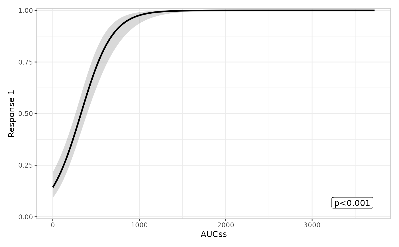

A worked example: the multi-parameter case

toy_emax’s three parameters (e0, emax, ec50) have no single “the” effect – there’s no term you could headline with a lone p-value without implying the other two don’t matter. This is exactly the coefficients-instead-of-p_value case the contract exists for:

er_summary.toy_emax <- function(model, ...) {
  s <- summary(model)$coefficients
  coefficients <- tibble::tibble(
    term = rownames(s),
    estimate = s[, "Estimate"],
    std_error = s[, "Std. Error"],
    statistic = s[, "t value"],
    p_value = s[, "Pr(>|t|)"]
  )
  list(p_value = NULL, coefficients = coefficients)
}

erglm_data |>
  er_plot(aucss, biomarker_change) |>
  er_plot_add_model(emax_mod) |>
  er_plot_add_summary(model = emax_mod, style = "coefficients") |> 
  plot()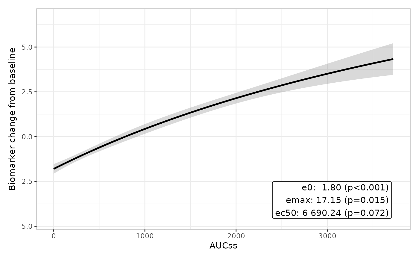

Note the explicit p_value = NULL above, and the explicit style = er_style_summary_coefficients on the er_plot_add_summary() call – er_style_summary_pvalue() is still the default summary builder regardless of which model is attached, and it would silently draw nothing here (correctly: it reads config$p_value, sees NULL, and has nothing to show) rather than falling back to coefficients on your behalf. Matching a model whose er_summary() populates coefficients with a builder that actually reads coefficients is left to you, the caller – er_summary()’s job is only to make the data available.

er_predict_survival(): the er_tte() model overlay

er_predict_survival(model, newdata, time_grid, conf_level = 0.95, ...)

Powers a single, specific thing: er_tte_add_model()’s parametric S(t) curve/ribbon, overlaid on a Kaplan-Meier estimate in the separate er_tte() mini-grammar (time on the x-axis, survival probability on the y-axis – see Time-to-event plots). It has nothing to do with er_plot()/er_vpc(); a model that implements er_predict()/ er_simulate()/er_summary() gets no benefit from also implementing this one, or vice versa.

The contract differs from er_predict()’s in one structural way: newdata carries one row per covariate profile (e.g. one row per stratification level), with no time column at all – times come from the separate time_grid argument instead. Return newdata cross-joined with time_grid (one row per newdata row × time_grid value), with three columns added: time, fit_survival (the point estimate of S(time | newdata row)), ci_lower, and ci_upper. Unlike er_predict()’s fit_resp, there’s no ambiguity about scale to get right here – a survival probability only ever has one scale, [0, 1].

There’s no NULL-returning default method, unlike er_simulate()/ er_summary(): a model with no survival-curve support should simply not implement this generic at all, and er_tte_add_model() errors informatively (naming the model’s class) if it’s called with one anyway.

A worked example

Suppose your modelling package fits parametric survival models via survival::survreg(). A Weibull or log-normal fit needs its own scale parameter accounted for, but the exponential case – where proportional hazards and accelerated failure time coincide – keeps the maths simple enough to work through by hand, so that’s what this example uses:

library(survival)

fit_toy_survival <- function(formula, data) {
  fit <- survreg(formula, data = data, dist = "exponential")
  class(fit) <- c("toy_survival", class(fit))
  fit
}

lung_sex <- lung |> transform(sex = factor(sex, labels = c("Male", "Female")))
mod_survival <- fit_toy_survival(Surv(time, status == 2) ~ sex, lung_sex)
class(mod_survival)
#> [1] "toy_survival" "survreg"

survreg()’s exponential model is an accelerated-failure-time model on the log-time scale, log(T) = X * beta + error, with error’s distribution fixed (no separate scale parameter to estimate, unlike Weibull/log-normal). That means S(t | x) = exp(-t * exp(-X * beta)), and coef(model)/vcov(model) already give you everything needed for both the point estimate and its uncertainty – no numerical delta method required, since the linear predictor X * beta enters S(t | x) through a strictly monotonic transform. That monotonicity is what lets the method below build a confidence interval by computing one for the linear predictor first, then mapping its two endpoints through S(t | x), rather than propagating a standard error through a nonlinear function the way er_predict.toy_emax() had to earlier in this article:

er_predict_survival.toy_survival <- function(model, newdata, time_grid, conf_level = 0.95, ...) {
  z <- -qnorm((1 - conf_level) / 2)

  X <- model.matrix(delete.response(terms(model)), data = newdata)
  beta <- coef(model)
  eta <- as.vector(X %*% beta)
  se_eta <- sqrt(rowSums((X %*% vcov(model)) * X))

  grid <- newdata[rep(seq_len(nrow(newdata)), each = length(time_grid)), , drop = FALSE]
  grid$time <- rep(time_grid, times = nrow(newdata))
  eta <- rep(eta, each = length(time_grid))
  se_eta <- rep(se_eta, each = length(time_grid))

  grid$fit_survival <- exp(-grid$time * exp(-eta))
  grid$ci_lower <- exp(-grid$time * exp(-(eta - z * se_eta)))
  grid$ci_upper <- exp(-grid$time * exp(-(eta + z * se_eta)))
  rownames(grid) <- NULL
  grid
}

That’s the whole method. Plugged into er_tte_add_model(), it overlays the fitted exponential curve (with its confidence band) on top of the Kaplan-Meier estimate for each stratum:

lung_sex |>
  er_tte(time, status == 2, stratify_by = sex) |>
  er_tte_add_curve() |>
  er_tte_add_model(mod_survival) |>
  plot()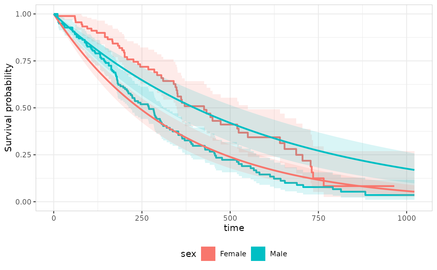

The exponential fit is visibly too smooth relative to the Kaplan-Meier step curve – a single constant hazard per stratum can’t reproduce the data’s own shape – which is exactly the kind of model-vs-data mismatch an S(t) overlay like this one exists to make visible. A Weibull or log-normal fit would track the step curve more closely, at the cost of an extra scale parameter this simplified method doesn’t handle – extending it that way is a reasonable next step for a real implementation, not covered here.

Testing your implementation

There’s no formal conformance checker for this interface – it’s four plain S3 generics, so the real test is simply exercising the layers that call them:

• er_plot_add_model(your_model) exercises er_predict() alone.
• er_plot_add_model(your_model, style = "spaghetti") additionally exercises er_simulate()’s fit_resp.
• er_vpc_add_simulated(model = your_model, ...) additionally exercises er_simulate()’s sim_resp.
• er_plot_add_summary(model = your_model) (paired with whichever summary builder matches what your er_summary() populates) exercises er_summary().
• er_tte_add_model(your_model) exercises er_predict_survival() – a separate check from the four above, since it belongs to the er_tte() grammar rather than er_plot()/er_vpc().

If you only implement er_predict(), that’s a complete, valid implementation – er_simulate()/er_summary() are additive, not phases of a single required rollout, and er_predict_survival() is unrelated to all three (it only matters if your model also has something to say about er_tte()’s time-to-event grammar). And if a method genuinely can’t do better than the default (NULL), leaving it unimplemented is the correct choice, not a gap to apologise for: every erplots builder that depends on er_simulate()/er_summary() already has to handle “not available” gracefully, since the default method returns NULL for every model class that hasn’t implemented one. er_predict_survival() is the one exception to that pattern – its default method errors rather than returning NULL, since there’s no plotting fallback for a survival curve nobody can compute.

If your method requires an argument beyond the fixed contract (like toy_landmark’s landmark_time above), remember that exercising it means passing predict_args/summary_args/simulate_args explicitly – calling er_plot_add_model(your_model) with no predict_args will correctly error if your method has no default for that argument, the same way toy_landmark’s did above.

Real-world implementations

The examples above are toy classes built for this article. Three real packages implement this interface for production modelling code, and are worth reading directly if you want to see the pattern applied to a less simplified model:

• erglm wraps glm()-based exposure-response models. Its er_predict.erglm_model() and er_simulate.erglm_model() methods follow the same shape as toy_model’s above (link-scale prediction with an inverse-link transform; a multivariate-normal draw over the coefficient vector for simulation) but handle all four families erglm supports (binomial/poisson/gaussian/Gamma), plus the auto-seed-and-report behaviour mentioned above. Its er_summary.erglm_model() populates all three keys at once (p_value for the exposure coefficient, coefficients for every term, glance for goodness-of-fit).
• emaxnls fits genuine Emax/sigmoidal models via nls(), and is the real-world analogue of toy_emax above: er_summary.emaxnls() always returns p_value = NULL and populates coefficients (one row per E0/Emax/ logEC50) instead, for exactly the reason discussed above – no single parameter is “the” effect. Its emax_logistic() variant fits a binary response but returns an object with class c("emaxlogistic", "emaxnls"), so it reuses the same three methods via ordinary S3 inheritance; the methods branch internally (on inherits(model, "emaxlogistic")) to keep predictions bounded in [0, 1] and to draw Bernoulli rather than Gaussian noise for sim_resp, rather than needing a fourth, separate set of methods.
• ertte implements the full interface for time-to-event models: er_predict()/er_simulate()/ er_summary() methods for scalar landmark-binary/RMST reductions of a survival curve (letting a time-to-event model plug into the ordinary er_plot()/er_vpc() grammar too), plus er_predict_survival.ertte_model() – wrapping its own ertte_predict() – for the full S(t) curve overlay er_tte_add_model() needs. Unlike toy_survival above, it handles the Weibull/log-normal scale parameter this article’s simplified exponential example sidesteps, via ertte_predict()’s own machinery rather than the from-scratch delta method used here.

All three are Suggests-only dependencies of erplots (see DESCRIPTION), used here only as worked examples – there’s no requirement to depend on any of them to implement this interface for your own model class.

See also

• ?er_model_interface for the terse, canonical statement of the contract this article expands on.
• The exposure-response plotting grammar for how er_predict()/ er_simulate()/er_summary()’s outputs flow into the layers that consume them (config$predictions, config$summary, config$p_value, and so on).
• Extending erplots if, once your model works with the built-in layers, you also want to change how a layer draws that model’s output – a different kind of extensibility from the one this article covers.
• Time-to-event plots for er_tte_add_model()’s overlay in action against a real implementation (ertte), and the rest of the er_tte() grammar it plugs into.