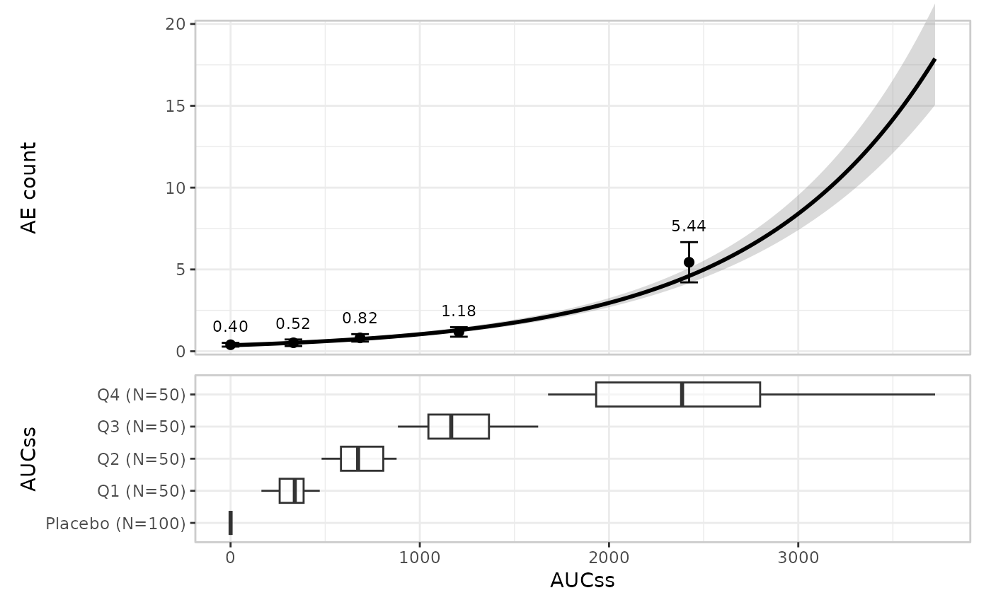
The erplots package supplies a mini-language for generating exposure-response plots commonly used in pharmacometric analyses. It is designed to be model agnostic, in the sense that it will work for any modelling tool that implements a few key interface functions (see Implementing the model interface). It can support binary response data, continuous response data, and count response data. This article focuses on count data, using a Poisson model fitted using the erglm package. It covers the substantive aspects of plot construction, not the superficial features like labels, palettes, and visual theme. Those are covered by the theming exposure-response plots article, which applies unchanged regardless of response type.
Fit the model first
mod_poisson <- erglm_model(ae_count ~ aucss, erglm_data, family = poisson())Count responses, such as an adverse-event count, auto-detect as
"continuous" under er_plot()’s
"auto" logic (they’re neither logical nor confined to
{0, 1}), and are summarised the same way a genuinely
continuous response is (bin mean plus t-interval) unless you declare
response_type = "count" explicitly.
Defining plots
erglm_data |>
  er_plot(aucss, ae_count) |>
  er_plot_add_model(mod_poisson) |>
  er_plot_add_quantiles() |>
  plot()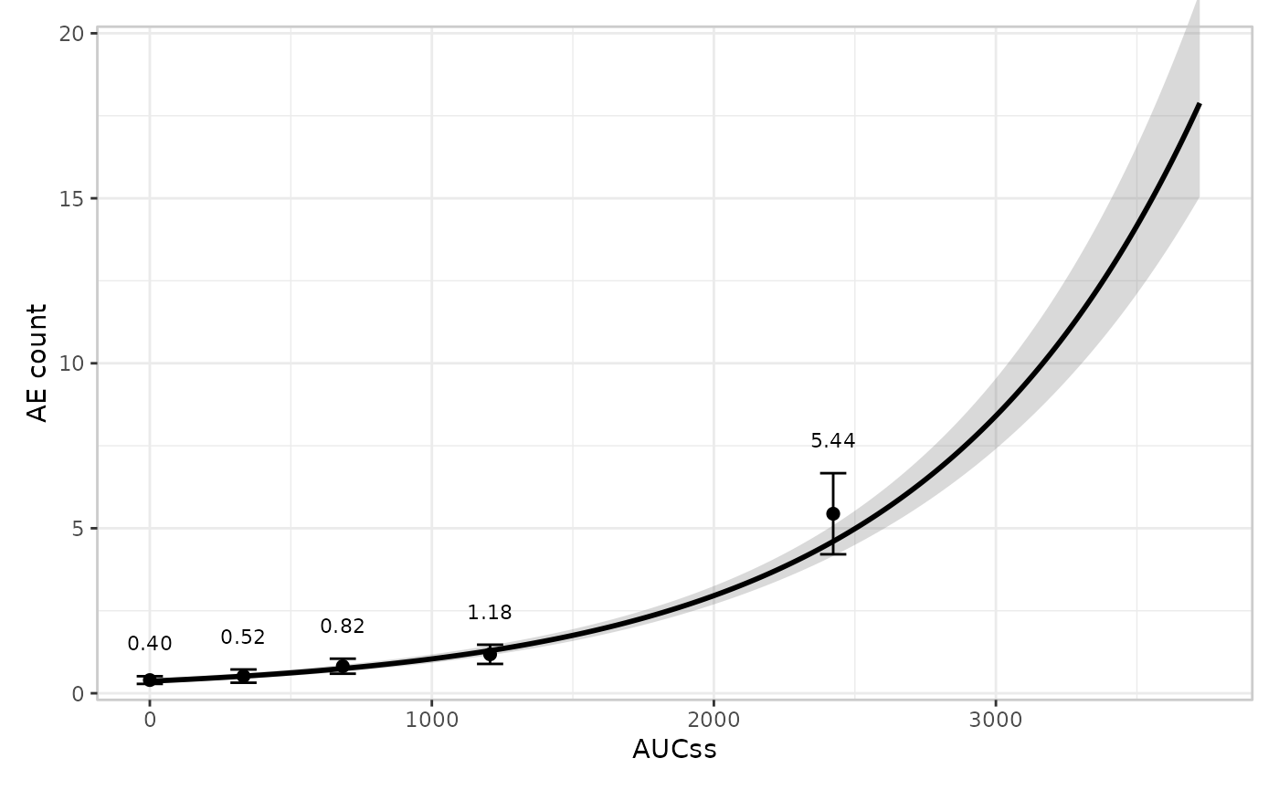
Stratification
Stratification adds colour across all layers, and requires a model
that includes the stratification variable as a term. See the binary responses article for
a fuller worked example, including how to suppress stratification for
specific layers with keep_strata = FALSE.
mod_poisson_sex <- erglm_model(
  ae_count ~ aucss + sex, erglm_data, family = poisson()
)

erglm_data |>
  er_plot(aucss, ae_count, stratify_by = sex) |>
  er_plot_add_model(mod_poisson_sex) |>
  er_plot_add_quantiles() |>
  er_plot_add_data() |>
  plot()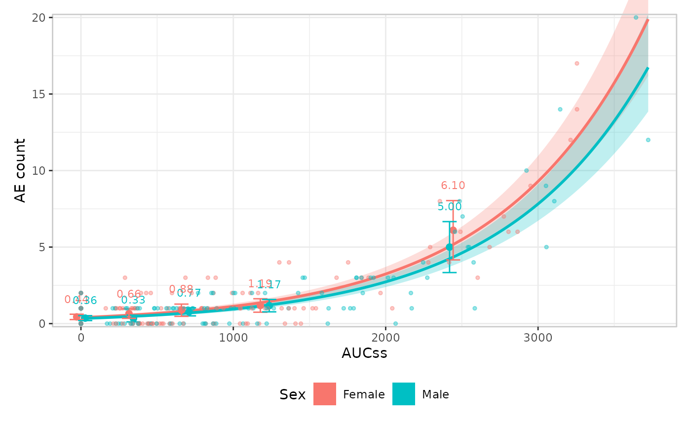
Model layer
The model layer doesn’t look at response_type at all –
it only consumes er_predict()/er_simulate()
output – so it works exactly the same way as for a binary response. See
the binary responses article
for er_style_model_spaghetti(); the default builder is used
here:
erglm_data |>
  er_plot(aucss, ae_count) |>
  er_plot_add_model(mod_poisson) |>
  er_plot_add_quantiles() |>
  plot()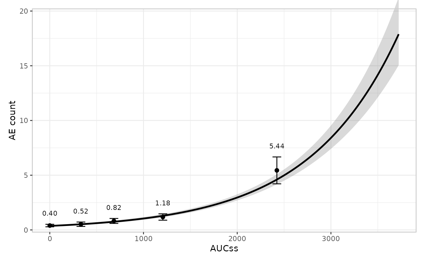
Summary layer
The summary layer doesn’t look at response_type at all
either – it only consumes whatever the model’s own
er_summary() method returns – so it works exactly the same
way as for a binary response. See the binary responses article for
er_style_summary_gof() and the full four-builder set; the
default builder is used here:
erglm_data |>
  er_plot(aucss, ae_count) |>
  er_plot_add_model(mod_poisson) |>
  er_plot_add_summary(model = mod_poisson) |>
  plot()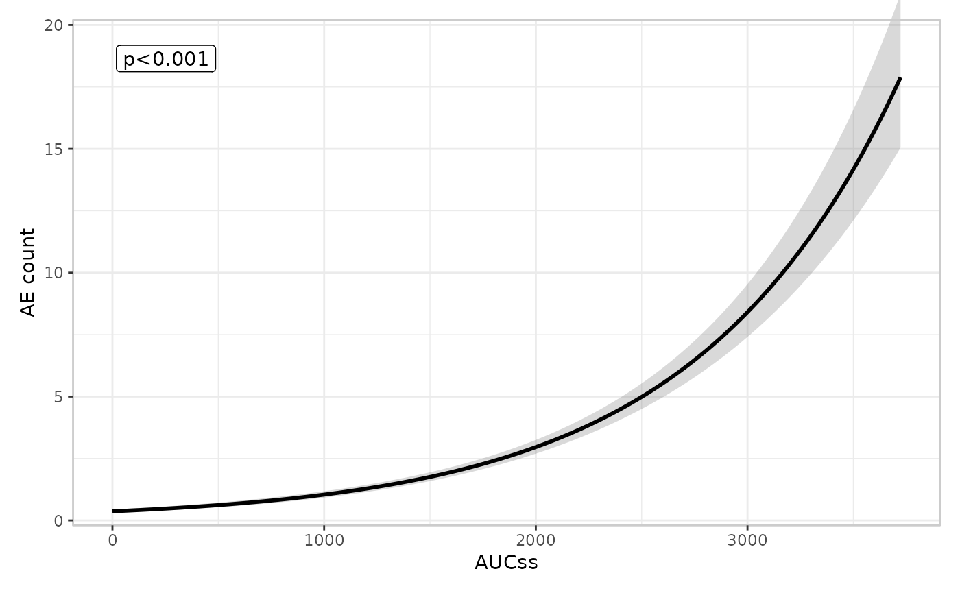
Quantile layer
Under auto-detection, a count response is summarised the same way a continuous response is – bin mean plus t-interval:
erglm_data |>
  er_plot(aucss, ae_count) |>
  er_plot_add_model(mod_poisson) |>
  er_plot_add_quantiles() |>
  plot()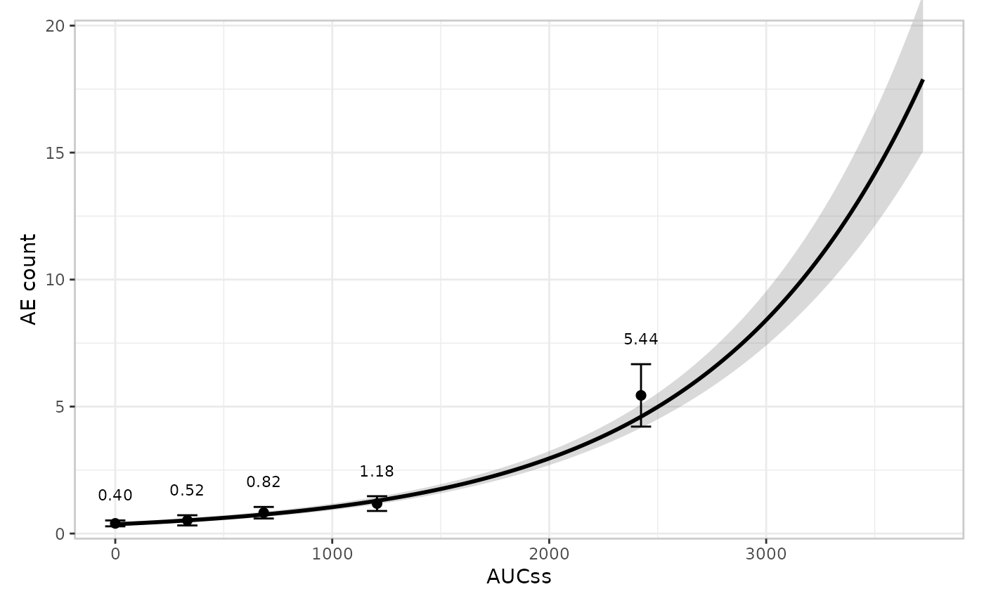
Declaring response_type = "count" swaps the t-interval
approximation for an exact Poisson interval (bin mean plus
ci_poisson() instead of ci_t()), which never
produces a negative lower bound – useful for low-count bins, where the
t-interval approximation can. For erglm_data’s own
ae_count, none of the bin means are low enough for this to
actually happen, so the two plots above would look almost identical if
you re-ran the last one with response_type = "count". To
make the difference concrete, here’s a synthetic dataset where the
placebo arm has only 2 events among 20 subjects:
set.seed(84)
placebo_counts <- rpois(20, 0.05)
while (sum(placebo_counts) != 2) placebo_counts <- rpois(20, 0.05)

aucss_dosed <- sort(runif(80, 100, 3000))
count_dosed <- rpois(80, 0.1 + 0.003 * aucss_dosed)

low_count_data <- data.frame(
  aucss = c(rep(0, 20), aucss_dosed),
  ae_count = c(placebo_counts, count_dosed)
)

mod_low_count <- erglm_model(ae_count ~ aucss, low_count_data, family = poisson())
The default (t-interval) path’s placebo-arm error bar dips visibly below zero – a nonsensical negative event rate:
low_count_data |>
  er_plot(aucss, ae_count) |>
  er_plot_add_model(mod_low_count) |>
  er_plot_add_quantiles() |>
  plot() +
  ggplot2::coord_cartesian(ylim = c(-0.5, 1.5), xlim = c(-50, 800))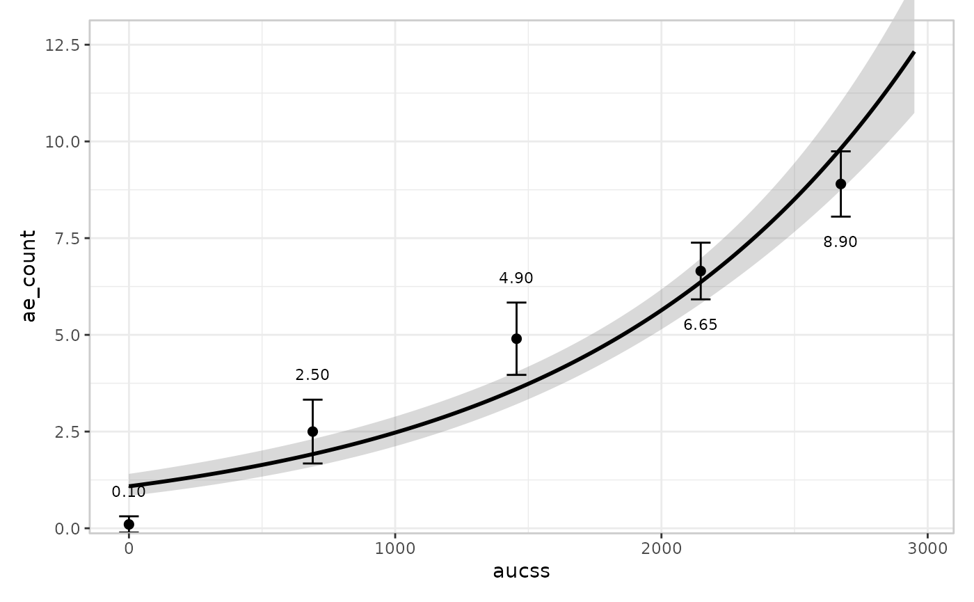
#> Coordinate system already present.
#> ℹ Adding new coordinate system, which will replace the existing one.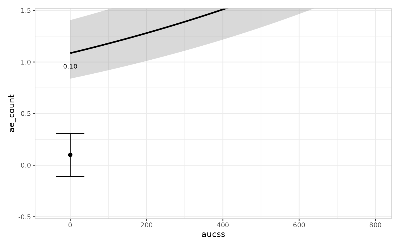
Declaring response_type = "count" keeps the same
placebo-arm point estimate but replaces the t-interval with an exact
Poisson interval, which stays non-negative:
low_count_data |>
  er_plot(aucss, ae_count, response_type = "count") |>
  er_plot_add_model(mod_low_count) |>
  er_plot_add_quantiles() |>
  plot() +
  ggplot2::coord_cartesian(ylim = c(-0.5, 1.5), xlim = c(-50, 800))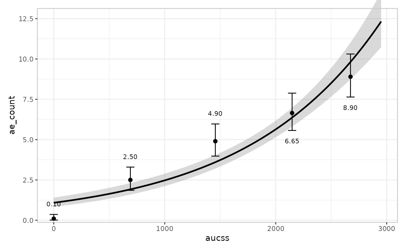
#> Coordinate system already present.
#> ℹ Adding new coordinate system, which will replace the existing one.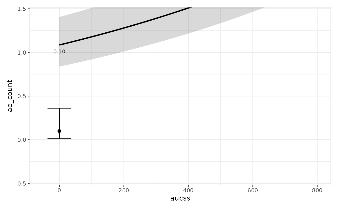
Data layer
er_plot_add_data() adds the raw observations at their
true (exposure, response) coordinates via
er_style_data_overlay(), the default builder for a count
response – no jitter is needed, since the response isn’t confined to
0/1. er_style_data_hex() (2D density via
geom_hex()) is also available for a count response; see
?er_style_data for details:
erglm_data |>
  er_plot(aucss, ae_count) |>
  er_plot_add_model(mod_poisson) |>
  er_plot_add_data() |>
  plot()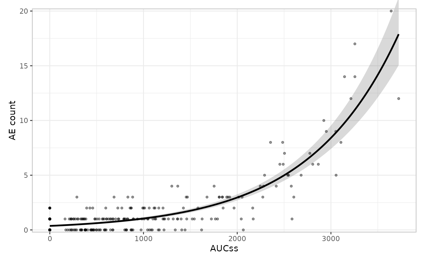
There’s no built-in panel-based alternative for a count response –
er_style_data_boxjitter() (the panel-based
responders/non-responders design covered in the binary
responses article) is binary-only. If you need a panel-based builder
here, you can write a custom one and tag it with
er_style_tag(fn, layout = "panel") – see the Extending erplots article.
Group layer
The group layer doesn’t look at response_type at all –
it only consumes the exposure variable – so it works exactly the same
way as for a binary response. See the binary responses article for
multiple grouping variables and er_style_group_violin();
the default builder and a single grouping variable are shown here:
erglm_data |>
  er_plot(aucss, ae_count) |>
  er_plot_add_model(mod_poisson) |>
  er_plot_add_quantiles() |>
  er_plot_add_groups(group_by = aucss) |>
  plot()