Add a quantile-binned response summary layer

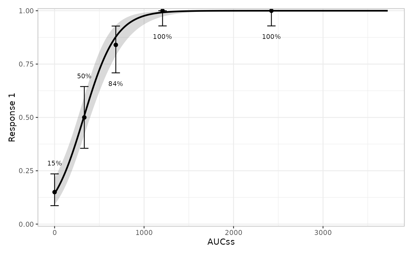
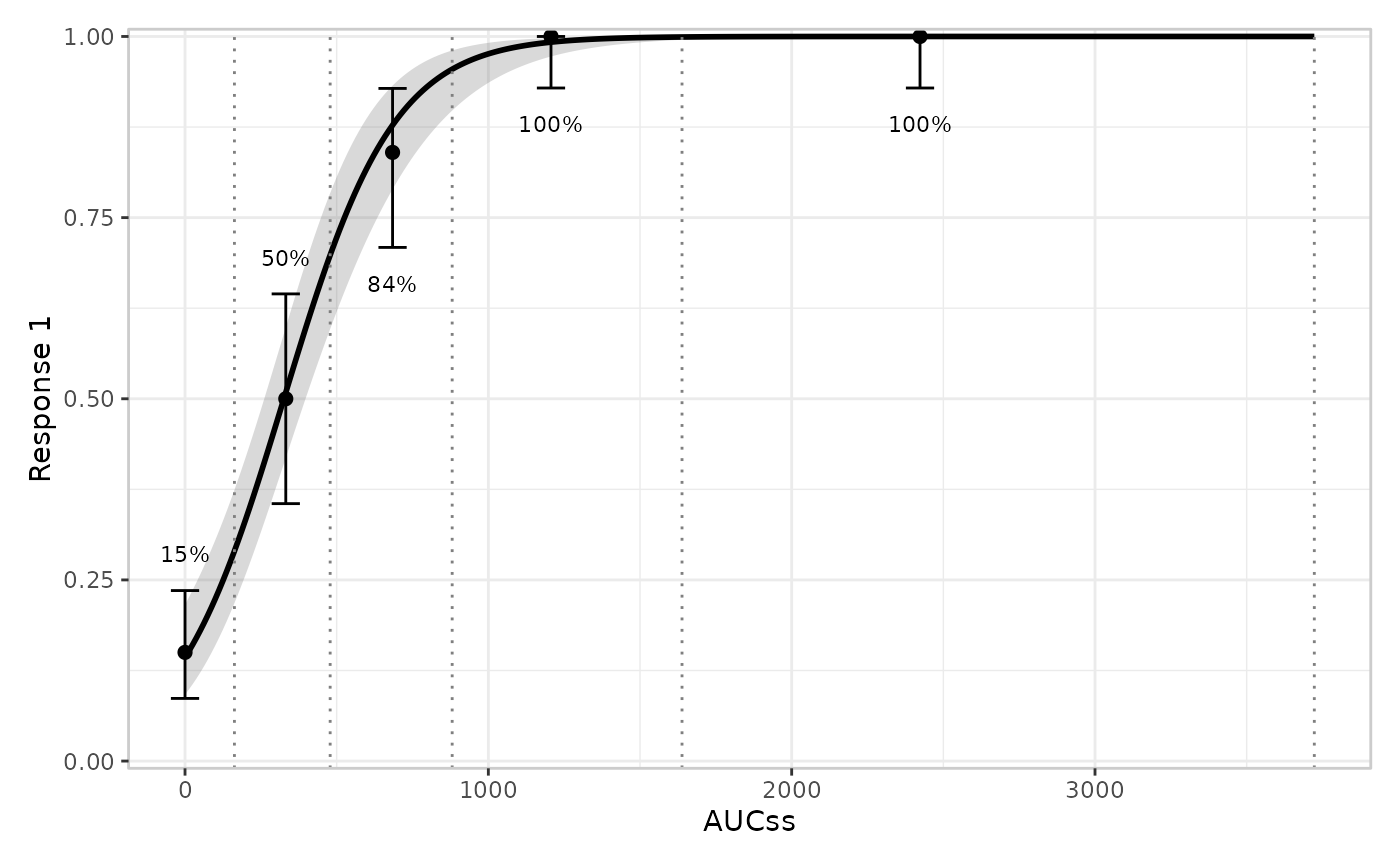
Adds the quantile layer: exposure is cut into quantile bins (see cut_exposure_quantile()) and, within each bin, the response is summarised with a point estimate and confidence interval.

Usage

er_plot_add_quantiles(
  object,
  keep_strata = NULL,
  style = NULL,
  bins = 4,
  conf_level = 0.95,
  ...
)

Arguments

object

Partially constructed plot, an er_plot object.

keep_strata

Logical, indicating whether this layer should be split by the plot's stratification variable; defaults to TRUE if stratify_by was set in er_plot(), FALSE otherwise.

style

Function drawing the quantile summary; defaults to er_style_quantile_errorbar() (point + error bar).

bins

Number of exposure bins (not counting placebo).

conf_level

Confidence level for the interval.

...

Additional named arguments forwarded, unchanged, to style when it's called at build time. Arguments must be named.

Value

The input object, with the quantile layer added.

Details

The type of confidence interval shown depends on the response_type set in er_plot():

• "binary": Clopper-Pearson interval (see ci_clopper_pearson())

• "continuous": Student t-interval (see ci_t())

• "count": exact Poisson interval (see ci_poisson())

Note that count responses are not automatically detected as such: they default to "continuous" and are summarised the same way as any other continuous response unless response_type = "count" is declared explicitly in er_plot().

See also

er_plot(), er_plot_add_model(), er_plot_add_summary(), er_plot_add_data(), er_plot_add_groups(), er_vpc(), er_style()

Examples

if (requireNamespace("erglm", quietly = TRUE)) {
library(erglm)
mod <- erglm_model(ae1 ~ aucss, erglm_data, family = binomial())
erglm_data |>
  er_plot(aucss, ae1) |>
  er_plot_add_model(mod) |>
  er_plot_add_quantiles() |>
  plot()

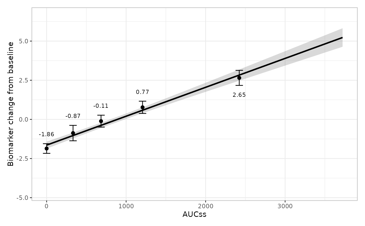
# continuous response: bin means/t-intervals instead of rates/
# Clopper-Pearson intervals, auto-detected from the response column
mod3 <- erglm_model(biomarker_change ~ aucss, erglm_data, family = gaussian())
erglm_data |>
  er_plot(aucss, biomarker_change) |>
  er_plot_add_model(mod3) |>
  er_plot_add_quantiles() |>
  plot()

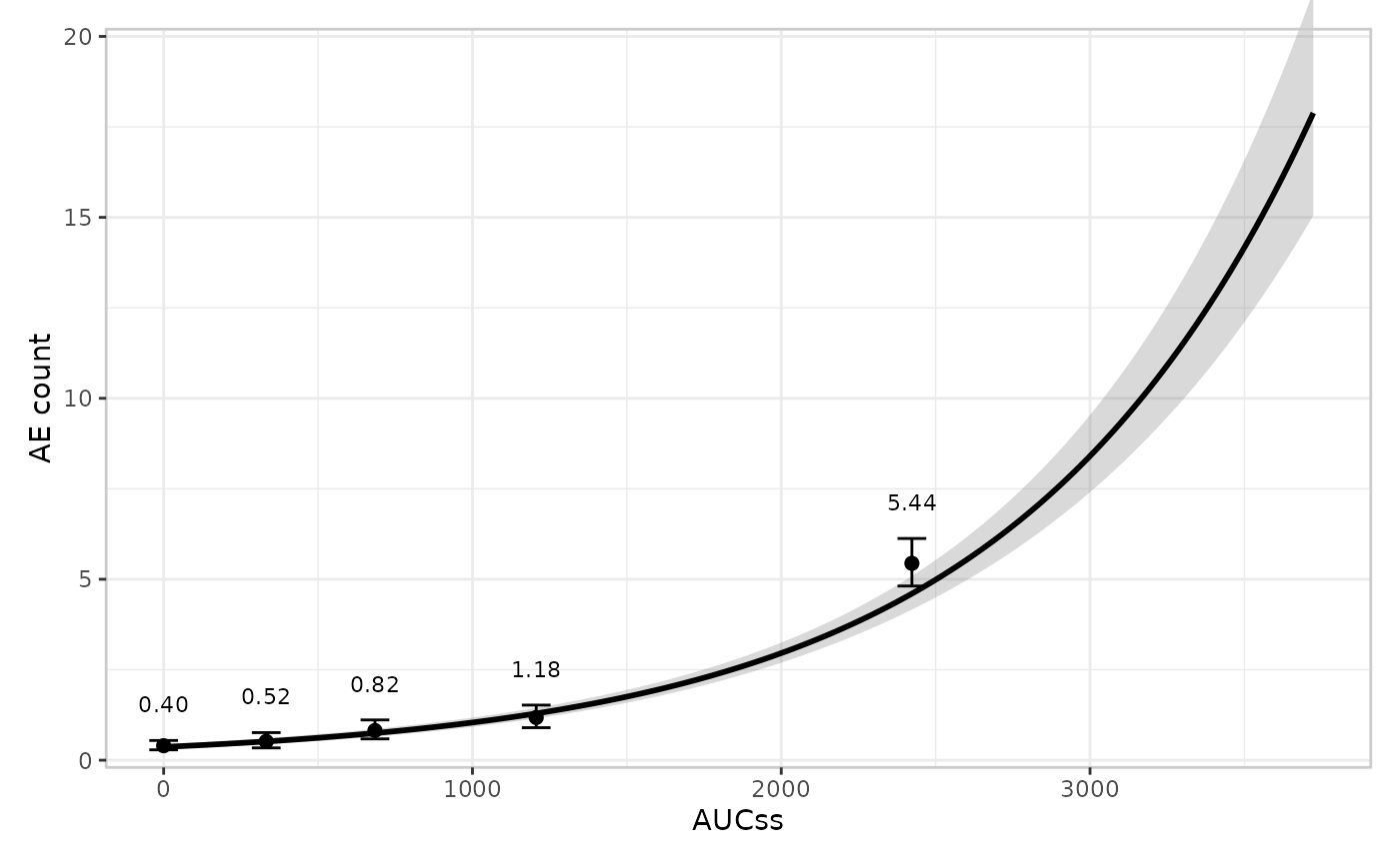
# count response: declare response_type = "count" explicitly for an
# exact Poisson interval instead of the t-interval approximation used
# by the auto-detected ("continuous") default
mod4 <- erglm_model(ae_count ~ aucss, erglm_data, family = poisson())
erglm_data |>
  er_plot(aucss, ae_count, response_type = "count") |>
  er_plot_add_model(mod4) |>
  er_plot_add_quantiles() |>
  plot()

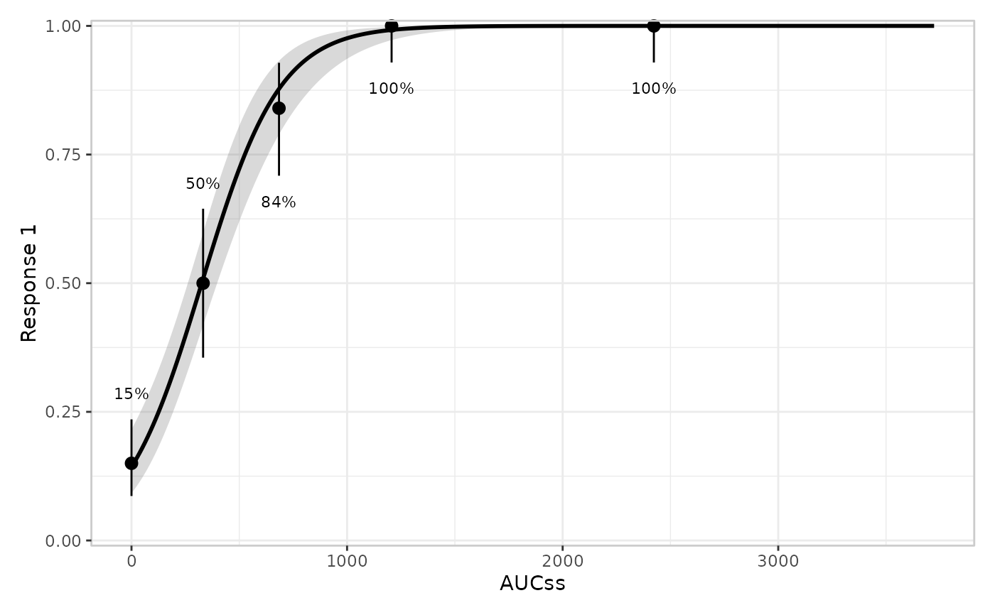
# a pointrange instead of the default errorbar
erglm_data |>
  er_plot(aucss, ae1) |>
  er_plot_add_model(mod) |>
  er_plot_add_quantiles(style = er_style_quantile_pointrange) |>
  plot()

# the default errorbar, with dotted lines marking the quantile-bin
# boundaries
erglm_data |>
  er_plot(aucss, ae1) |>
  er_plot_add_model(mod) |>
  er_plot_add_quantiles(style = er_style_quantile_errorbar_vlines) |>
  plot()

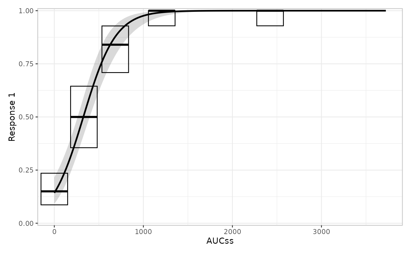
# plug in a fully custom builder; see `?er_style`
build_quantile_crossbar <- function(data, config, stratify, exposure,
                                     response, strata, theme, ...) {
  ggplot2::geom_crossbar(
    data = config$summary,
    mapping = ggplot2::aes(x = x_mid, y = y_mid, ymin = ci_lower, ymax = ci_upper),
    inherit.aes = FALSE
  )
}
erglm_data |>
  er_plot(aucss, ae1) |>
  er_plot_add_model(mod) |>
  er_plot_add_quantiles(style = build_quantile_crossbar) |>
  plot()
}