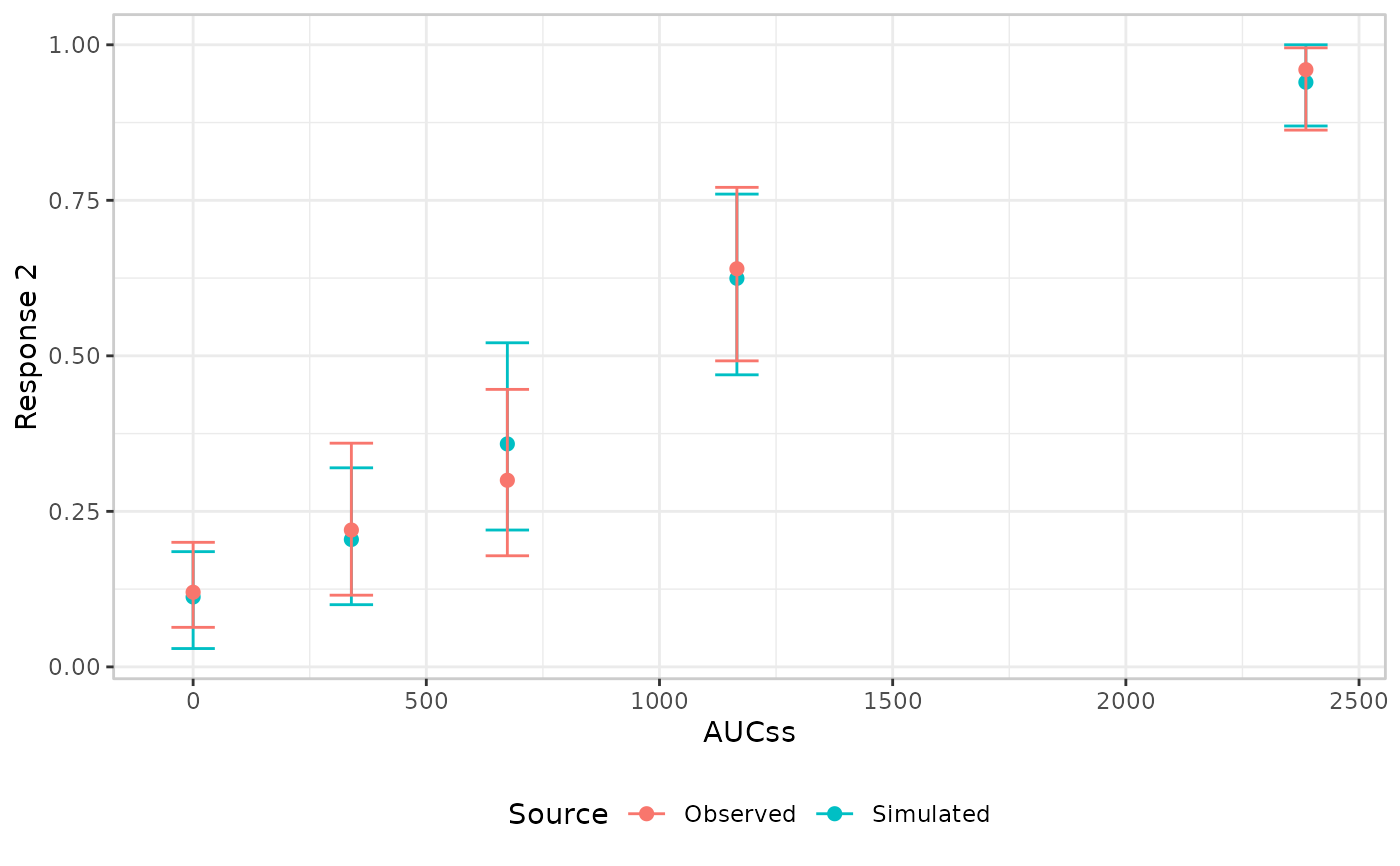
The exposure-response VPC mini-language

Create an er_vpc specification for a visual predictive check. Build the plot by adding an observed layer and a simulated layer, and render with plot()/print() or er_vpc_build().

Usage

er_vpc(
  data,
  exposure,
  response,
  response_type = "auto",
  plot_by = NULL,
  n_bins = 4,
  stratify_by = NULL,
  n_strata = 4,
  conf_level = 0.95,
  probs = c(0.1, 0.5, 0.9)
)

Arguments

data: Data frame or tibble containing the observed data.
exposure: Exposure variable (one variable, unquoted).
response: Response variable (one variable, unquoted).
response_type: One of "auto", "binary", "continuous", or "count".
plot_by: Variable (unquoted) plotted on the x-axis and used to bin/group the observed vs. simulated comparison. Defaults to exposure. A numeric variable is split into n_bins quantile bins (placebo, i.e. 0, kept in its own bin when plot_by is the exposure variable itself); a categorical variable is used as-is, with no binning.
n_bins: Number of quantile bins, when plot_by is numeric.
stratify_by: Optional variable (unquoted) splitting the VPC into one facet panel per level, via ggplot2::facet_wrap(). A categorical variable is used as-is; a numeric variable is automatically split into n_strata quantile bins (placebo, i.e. 0, kept in its own bin when stratify_by is the exposure variable itself), with a message reporting that this happened. Must resolve to a different variable than plot_by. Defaults to NULL (no faceting, a single panel, matching prior behaviour).
n_strata: Number of quantile bins, when stratify_by is numeric. Ignored when stratify_by is NULL or categorical.
conf_level: Confidence level for both the observed- and simulated-side intervals. Must be strictly between 0 and 1.
probs: Percentiles to compute for a percentile-based builder (e.g. er_style_vpc_observed_quantile_line()/er_style_vpc_simulated_quantile_ribbon()/ er_style_vpc_observed_quantile_errorbar()/er_style_vpc_simulated_quantile_errorbar(); ignored by the default adaptive mean/errorbar pair). Only computed for a continuous/count response.

Value

An (empty) plot object of class er_vpc.

Details

er_vpc_add_observed() bins the observed data and computes its response summary; er_vpc_add_simulated() must be added afterwards, since it reuses the observed layer's own binning decision so both sides share identical bin boundaries. Both layers are singletons (a second call replaces the previous one).

Unlike er_plot(), er_vpc() has no stratification concept and always renders a single panel – see er_vpc_add_observed() for plot_by, the (orthogonal) variable plotted on the x-axis and used to bin/group the comparison. Whether plot_by is "continuous" (numeric, quantile-binned) or "discrete" (used as-is) is auto-detected from the column's type and stored on object$group$type, mirroring how object$response$type records the response's type.

Examples

if (requireNamespace("erglm", quietly = TRUE)) {
library(erglm)
mod <- erglm_model(ae2 ~ aucss + sex, erglm_data, family = binomial())

erglm_data |>
  er_vpc(aucss, ae2, plot_by = aucss) |>
  er_vpc_add_observed() |>
  er_vpc_add_simulated(model = mod, seed = 9984) |>
  plot()
}