Add a raw-data layer

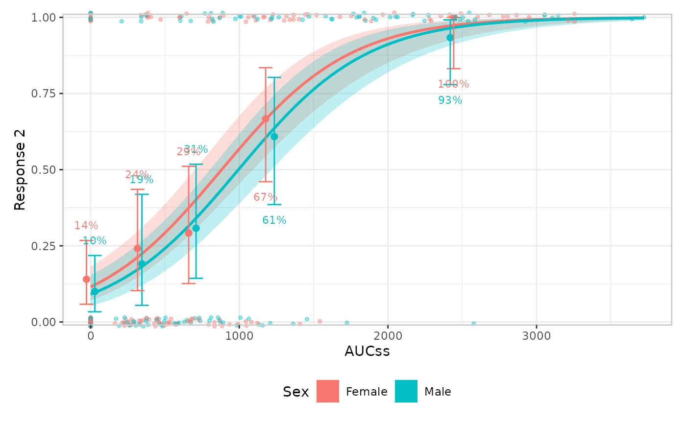
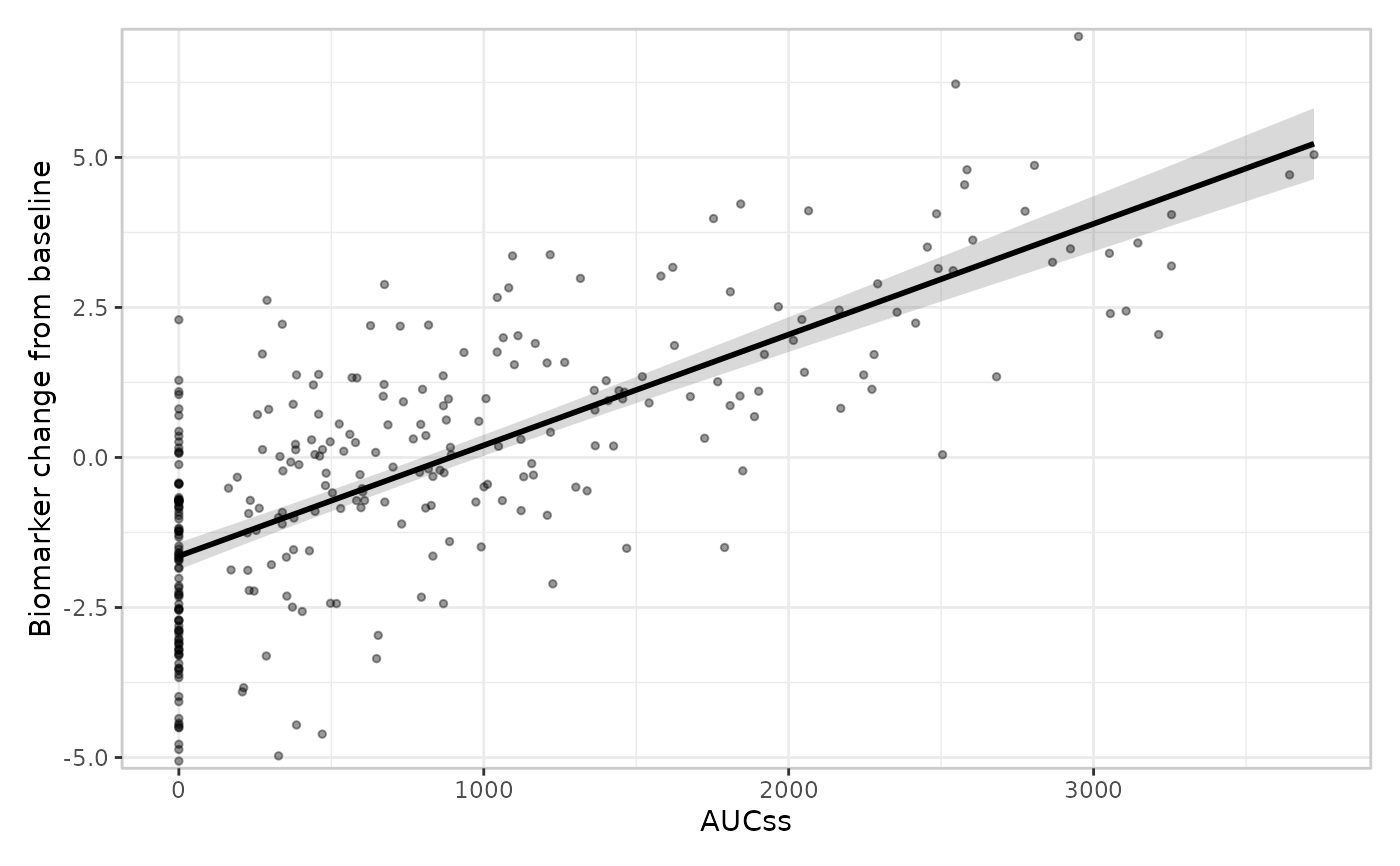
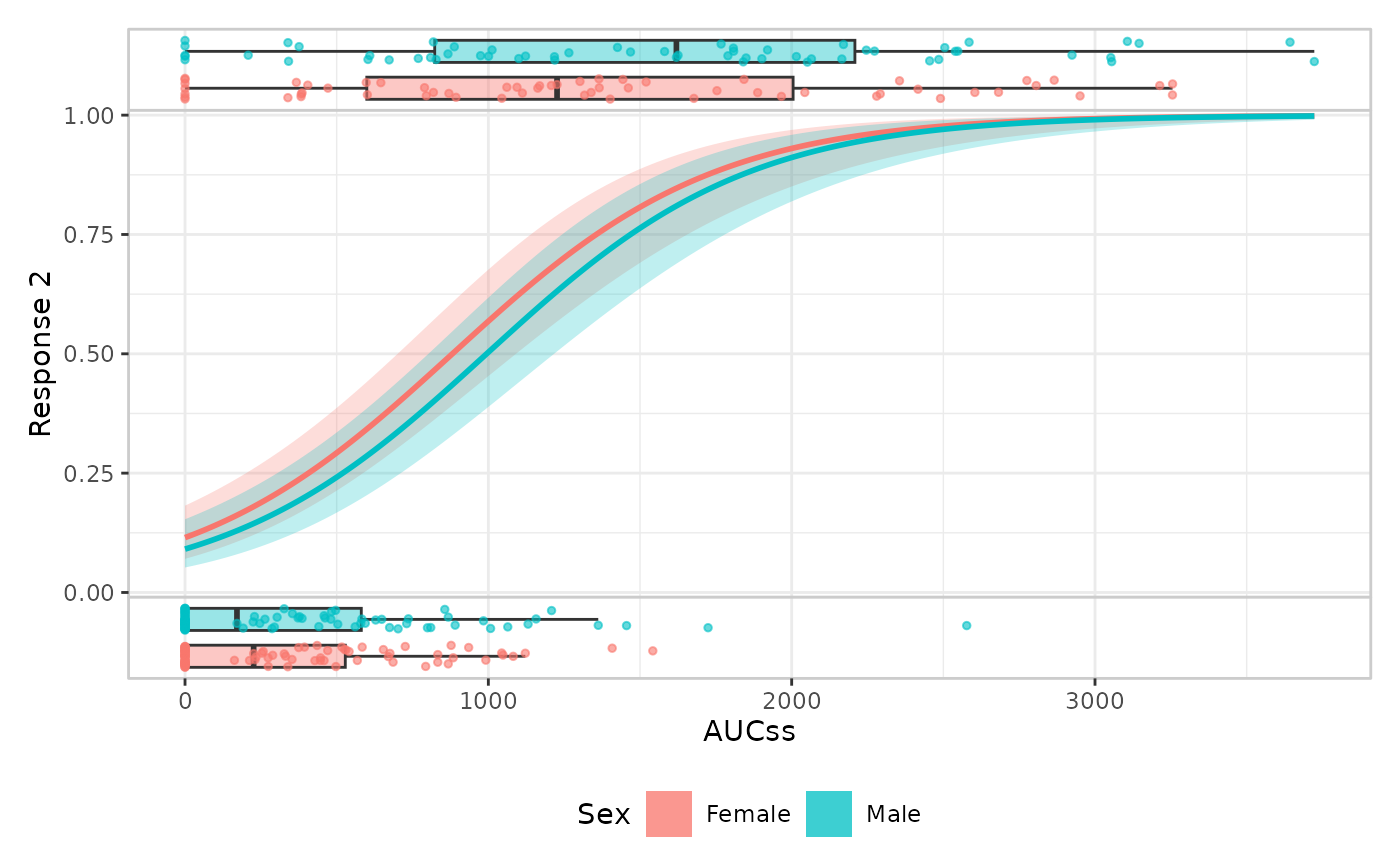
Adds the data layer: individual observations. By default, points are drawn as an overlay showing the exposure and response values in the main panel of the plot, but other possibilities are available.

Usage

er_plot_add_data(object, keep_strata = NULL, style = NULL, panel = "both", ...)

Arguments

object

Partially constructed plot (has S3 class er_plot).

keep_strata

Logical, indicating whether this layer should be split by the plot's stratification variable; defaults to TRUE if stratify_by was set in er_plot(), FALSE otherwise. See "Details" for how this interacts with a builder's structural family.

style

Function drawing the data layer – defaults to er_style_data_overlay(). Any function matching the standard (data, config, stratify, exposure, response, strata, theme, ...) signature and tagged with er_style_tag() can be supplied instead; see er_style() and "Details".

panel

Character string: "upper", "lower", or "both" (the default). Only meaningful for er_style_data_boxjitter() on a binary response; see "Details" for when "both" is required.

...

Additional named arguments forwarded, unchanged, to style when it's called at build time – see er_style()'s "Passing extra arguments to a builder" section. Must be named.

Value

The input object, with the data layer added.

Details

The default builder for the data layer is er_style_data_overlay(), which creates a plain scatter plot for continuous/count responses, or a scatter with a small vertical jitter for a binary response (whose y-values are exactly 0/1 and would otherwise overplot into two solid lines). This works uniformly across all three response types, with no response-type dispatch on which builder to use. er_style_data_boxjitter() instead uses a panel-based design, and is binary-response-only: responders (response == 1) get a boxplot + jittered points in an upper panel and non-responders (response == 0) get the same in a lower panel, so the panel shows the exposure distribution conditional on response, not just raw points. There is no built-in "panel"-layout builder for a continuous/count response; panel must be "both" (the default) for these response types regardless of builder, since there's no upper/lower partition to select from.

Every data-layer builder declares which of these two structural families it belongs to via er_style_tag() – "overlay" (a single call merged into the main panel) or "panel" (one-or-more panels stacked below the base plot) – which er_plot_add_data() reads off style to decide how to assemble the layer, rather than taking a separate argument for it. This makes the pairing structural rather than incidental: er_style_data_overlay() can never be routed into upper/lower panels, and er_style_data_boxjitter() can never be merged into the main panel. See er_style_tag() and er_style() for how to tag a custom builder the same way. If style is tagged with a layer other than "data", er_plot_add_data() errors informatively; an untagged builder is never checked (only layout is a hard requirement).

keep_strata's effect also depends on a builder's structural family: for an "overlay"-layout builder it always means a shared colour aesthetic, for any response type; for a "panel"-layout builder on a continuous/count response it instead produces one panel per stratum level rather than a shared colour aesthetic. panel must be "both" for an "overlay"-layout builder (there's no upper/lower partition to select from) and for a continuous/count response under a "panel"-layout builder (same reason).

See also

er_plot(), er_plot_add_model(), er_plot_add_summary(), er_plot_add_quantiles(), er_plot_add_groups(), er_style()

Examples

if (requireNamespace("erglm", quietly = TRUE)) {
library(erglm)
mod2 <- erglm_model(ae2 ~ aucss + sex, erglm_data, family = binomial())
erglm_data |>
  er_plot(aucss, ae2, stratify_by = sex) |>
  er_plot_add_model(mod2) |>
  er_plot_add_quantiles() |>
  er_plot_add_data() |>
  plot()

# continuous response: overlay works the same way, with no
# response-type-specific styling needed
mod3 <- erglm_model(biomarker_change ~ aucss, erglm_data, family = gaussian())
erglm_data |>
  er_plot(aucss, biomarker_change) |>
  er_plot_add_model(mod3) |>
  er_plot_add_data() |>
  plot()

# panel-based design, binary-response only: a boxplot + jittered
# points per panel (responders above, non-responders below), instead
# of an overlay in the main panel
erglm_data |>
  er_plot(aucss, ae2, stratify_by = sex) |>
  er_plot_add_model(mod2) |>
  er_plot_add_data(style = er_style_data_boxjitter) |>
  plot()

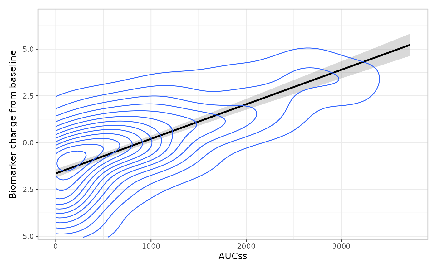
# plug in a 2D density in the main panel instead of a scatter; tagging
# it "overlay" via `er_style_tag()` keeps it in the single main-panel
# layout -- see `?er_style`
build_data_density <- er_style_tag(
  function(data, config, stratify, exposure, response, strata, theme, ...) {
    ggplot2::geom_density_2d(
      data = data,
      mapping = ggplot2::aes(x = .data[[exposure$name]], y = .data[[response$name]])
    )
  },
  layout = "overlay"
)
erglm_data |>
  er_plot(aucss, biomarker_change) |>
  er_plot_add_model(mod3) |>
  er_plot_add_data(style = build_data_density) |>
  plot()
}