erplots

erplots provides a fluent mini-language for building exposure-response plots: model curves/ribbons, quantile-binned response-rate summaries, data strips, and grouped distribution panels. It is model-agnostic: erplots never fits a model itself. Instead, you fit a model with whatever package suits your workflow (e.g. erglm for logistic regression), and pass the fitted object to er_plot_show_model(). Any model that implements er_predict() can be visualised; implementing er_simulate() and er_summary() additionally enables uncertainty spaghetti plots/VPCs and summary annotations (e.g. p-values). See ?er_model_interface.

Installation

You can install the development version of erplots like so:

pak::pak("djnavarro/erplots")

Example

library(erplots)
library(erglm)

mod <- erglm_model(ae1 ~ aucss, erglm_data, family = binomial())

erglm_data |> 
  er_plot(aucss, ae1) |> 
  er_plot_show_model(mod) |> 
  er_plot_show_quantiles() |> 
  er_plot_show_groups(aucss) |> 
  plot()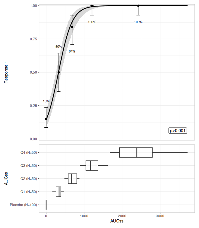

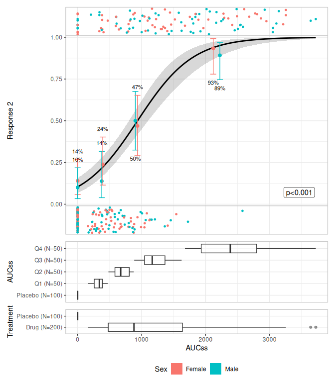
mod2 <- erglm_model(ae2 ~ aucss + sex, erglm_data, family = binomial())
mod2_marginal <- erglm_model(ae2 ~ aucss, erglm_data, family = binomial())

plt <- erglm_data |> 
   er_plot(aucss, ae2, stratify_by = sex) |> 
   # keep_strata = FALSE needs a model without the stratification
   # variable as a term, so we pass `mod2_marginal` here
   er_plot_show_model(mod2_marginal, keep_strata = FALSE) |> 
   er_plot_show_quantiles(bins = 3) |> 
   er_plot_show_datastrip() |> 
   er_plot_show_groups(group_by = c(aucss, treatment), keep_strata = FALSE)

print(plt)
#> <er_plot>
#>   plot variables:
#>     - exposure:        aucss
#>     - response:        ae2
#>     - stratification:  sex
#>   plot components:
#>     - model:           erglm_model/glm/lm
#>     - quantile:        3 bins
#>     - strip:           jitter both
#>     - group:           .aucss_quantile, treatment
#>   plots built: <none>
#>   output built: no
plot(plt)

VPC plots

sim <- erglm_vpc_sim(mod2, seed = 1234)
sim
#> # A tibble: 30,000 × 5
#>      ae2 aucss sex    row_id sim_id
#>    <int> <dbl> <fct>   <int>  <int>
#>  1     0  673. Male        1      1
#>  2     1 2806. Female      2      1
#>  3     0    0  Female      3      1
#>  4     0 1169. Female      4      1
#>  5     1  377. Male        5      1
#>  6     0  327. Female      6      1
#>  7     0    0  Male        7      1
#>  8     0 1208. Female      8      1
#>  9     0    0  Male        9      1
#> 10     0  254. Female     10      1
#> # ℹ 29,990 more rows

er_vpc_plot(erglm_data, sim, aucss, ae2, group_by = aucss)

er_vpc_plot(erglm_data, sim, aucss, ae2, group_by = sex)