Adjust theme/labels for a time-to-event plot

Set axis/legend labels, plot titles/captions, axis limits, theme objects, formatters, the legend key glyph, and relative panel heights for a time-to-event plot. This does not change which variable is mapped to which aesthetic – that's the builder's job via style (see er_style_tte_curve).

Usage

er_tte_theme(
  object,
  xlab = NULL,
  ylab = NULL,
  strata_lab = NULL,
  title = NULL,
  subtitle = NULL,
  caption = NULL,
  xlim = NULL,
  ylim = NULL,
  theme_base = NULL,
  theme_extra = NULL,
  format_p = NULL,
  format_percent = NULL,
  format_number = NULL,
  draw_key = NULL,
  height_curve = NULL,
  height_risktable = NULL
)

Arguments

object: Partially constructed plot (has S3 class er_tte).
xlab: Time axis label (single string). See "Details" for why xlim (not this) drives layout decisions; xlab is purely cosmetic.
ylab: Survival-probability axis label (single string).
strata_lab: Stratification legend label (single string). Errors if stratify_by wasn't set in er_tte() – there's no stratification legend to label.
title, subtitle, caption: Plot-level annotation text (single strings).
xlim: Time-axis limits (length-2, increasing numeric vector, no NA) – overwrites object$time$limits. See "Details" for the call-order caveat.
ylim: Survival-probability axis limits (length-2, increasing numeric vector, no NA). Purely cosmetic; defaults to c(0, 1).
theme_base: A ggplot2 theme object (e.g. ggplot2::theme_minimal()) – the swappable overall visual theme, defaulting to ggplot2::theme_bw().
theme_extra: A ggplot2 theme object (e.g. from ggplot2::theme()) with additional theme tweaks layered on top of theme_base. See "Details" for its default and replacement semantics.
format_p: Formatter function (typically from scales::label_pvalue()), used by er_tte_add_summary()'s log-rank annotation.
format_percent: Formatter function (typically from scales::label_percent()), used by er_style_tte_risktable_text()'s show_percent argument to format a risk-table count as a percentage of its stratum's baseline size.
format_number: Formatter function (typically from scales::label_number()), used by er_tte_add_summary()'s er_style_tte_summary_coefficients()/er_style_tte_summary_gof() builders to format coefficient/goodness-of-fit values.
draw_key: A key-glyph function (e.g. ggplot2::draw_key_point()), passed as the curve/model layers' key_glyph argument.
height_curve, height_risktable: Relative panel heights (single positive numbers), used when er_tte_add_risktable()'s panel is stacked below the curve panel. Supplying only one leaves the other unchanged.

Value

The input object, with the requested theme fields updated.

Details

Every argument defaults to NULL, meaning "leave whatever was set before unchanged". This allows repeated calls to er_tte_theme() to update only the supplied fields, like ggplot2::theme(). There is no implicit way to reset a field to the er_tte() default.

xlim overwrites object$time$limits directly (the same structural field er_tte() itself sets from the data), rather than a purely cosmetic ggplot2::coord_cartesian() zoom – mirroring er_plot_theme()'s own xlim (not er_vpc_theme()'s, which is display-only). This matters because object$time$limits also drives non-cosmetic defaults computed at add-layer time: er_tte_add_model()'s default time_grid and er_tte_add_risktable()'s default times both span it. Call er_tte_theme(xlim = ...) before those layers when you want the narrower/wider range reflected in their defaults; calling it after only changes the curve panel's own x-axis display. ylim, by contrast, is purely cosmetic (survival probability is always modelled on [0, 1]; this only changes what's displayed), stored on object$theme$ylim and defaulting to c(0, 1).

theme_extra defaults to a panel border plus legend.position = "bottom". Supplying a new value fully replaces this default rather than merging with it, so re-include the border/legend-position settings too if you want to keep them alongside your own additions.

title/subtitle/caption are applied via a single ggplot2::labs() call on the curve panel – unlike er_plot_theme()'s patchwork::plot_annotation() indirection, this is enough even when er_tte_add_risktable()'s panel is stacked below it via patchwork::wrap_plots(), since the curve panel is always the top-most one.

Examples

library(survival)
lung |>
  er_tte(time, status == 2) |>
  er_tte_add_curve() |>
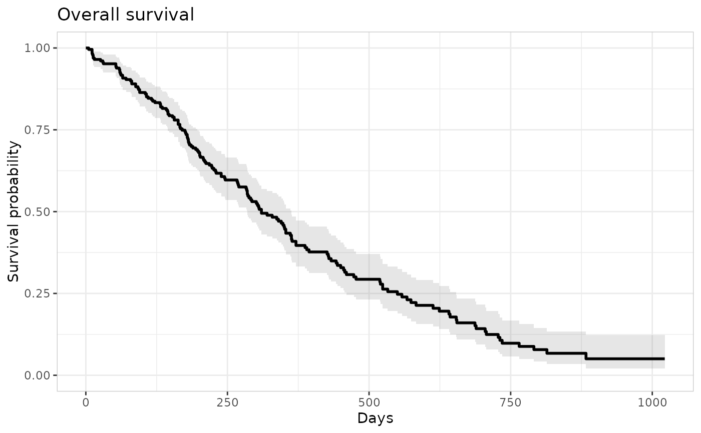
  er_tte_theme(
    xlab = "Days", ylab = "Survival probability",
    title = "Overall survival"
  ) |>
  plot()